Automatic differentiation computes gradients by representing a mathematical expression as a directed computational graph. Nodes hold variables or operations, while edges carry intermediate values. Deep-learning frameworks use this graph to differentiate a loss with respect to trainable parameters, supporting neural-network training. section 8.2.1
A logistic-regression workflow makes the process concrete: inputs and parameters produce a score, the score becomes a sigmoid prediction, and the prediction is compared with a target to form a loss. Setting requires_grad=True on weights and bias lets PyTorch track them; calling loss.backward() computes their gradients. An optimizer can then use those gradients to adjust parameters and reduce error. section 8.2.1
PyTorch logistic regression
With x = [1.0, 2.0, 3.0], trainable w and b, compute z = sum(x * w) + b, apply sigmoid, calculate binary cross-entropy against target 1.0, and call loss.backward() to print gradients for w and b. section 8.2.1
Figure 8.6 Example of a computational graph at a high level of abstraction.
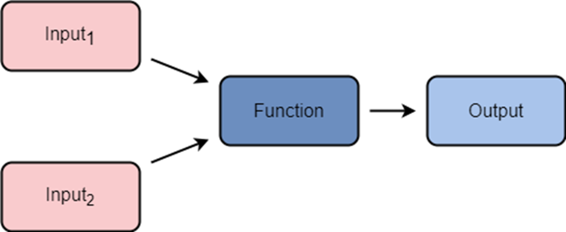
Use the computational-graph view to trace data from inputs through operations to a prediction and loss. section 8.2.1