Suppose you want to estimate the proportion of people who prefer tea. The proportion could be anywhere between 0 and 1, and a single estimate would hide your uncertainty. A beta distribution describes which values in that range you consider more plausible. Its shape is controlled by two hyperparameters, α and β. section 3.7
Beta(1, 1) is uniform: before seeing data, it gives equal density across the range. Other choices express different beliefs. Beta(0.5, 0.5), for example, favors values near the extremes rather than the middle. Choosing a prior matters most visibly when comparing how different starting beliefs respond to the same data. section 3.9
Updating a tea-preference estimate
Start with a Beta(1, 1) prior. If 3 of 5 people prefer tea, add the 3 successes to α and the 2 remaining trials to β. The posterior is Beta(4, 3), with a peak at 0.6. More generally, a Beta(α, β) prior and k successes in n trials give a Beta(α + k, β + n − k) posterior. section 3.7
This is a conjugate update: a beta prior combined with a binomial likelihood produces another beta distribution. Unlike a grid of candidate proportions, the continuous model does not require rounding or binning possible values. Probabilities over ranges come from areas under its density curve. section 3.18 section 3.7
Figure 3.3 Comparison between the posterior distributions of 𝑝 under different prior distributions.
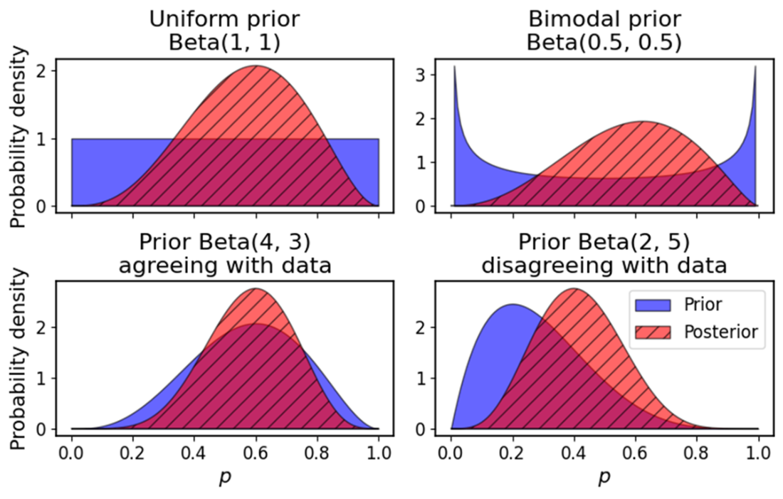
Compare the posterior curves under several beta priors: agreement with the data sharpens the peak, while conflicting beliefs produce a compromise. section 3.9
A posterior beta distribution can answer a decision-relevant question, not just supply a peak. For a modeled conversion rate, the probability of exceeding 0.1 is the area under the posterior density from 0.1 to 1. With posterior hyperparameters 64 and 438, that probability is about 0.97. It informs a launch decision, though the decision also depends on the costs and benefits of each action. section 11.10
from scipy.stats import beta
1 - beta(a, b).cdf(0.1)
Use SciPy’s beta cumulative distribution function to calculate the posterior probability that a conversion rate exceeds 0.1. section 11.10



