Beta distribution

As explained in Grokking Statistics

A continuous probability distribution over probabilities of success, parameterized by the observed numbers of successes and failures.

A beta distribution describes which underlying success rates are most likely after observing successes and failures. With 7 successes and 3 failures, alpha = 7 and beta = 3. section 3.8

Unlike the binomial distribution, which models a count of successes, the beta distribution models the continuous range of possible success rates from 0 to 1. Its smooth curve shows probability density, not probability directly; the total area under the curve is 1. section 3.12 section 3.8

Estimating a success rate

Suppose a manufacturer records 7 successes and 3 failures. Use SciPy to draw the beta density and calculate the area between success rates of 0.4 and 0.7: from scipy.stats import beta a, b = 7, 3 area = beta.cdf(0.7, a, b) - beta.cdf(0.4, a, b) print(area) # 0.437796414 The result is the area under the curve between 0.4 and 0.7, providing a way to examine how plausible that range of underlying success rates is given the observations. section 3.8

Figure 3.6 The beta distribution showing probabilities of success rates for a single trial

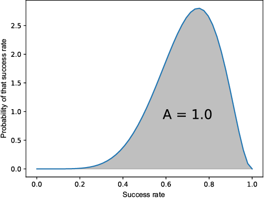
View the smooth beta-distribution curve for the possible success rates. section 3.8

How Grokking Statistics covers it

How deep it goes

Explains parameters, continuous density curves, unit area, and interval areas calculated with a cumulative distribution function.

Examples

Uses 7 successes and 3 failures, a SciPy density plot, and the interval from 0.4 to 0.7.

What it assumes

Assumes basic success-and-failure trials while teaching alpha and beta as observed successes and failures.

What you can do after

Apply it via SciPy to plot success-rate density and calculate the area within a chosen probability range.

How it connects

Connects success-rate estimation with binomial distributions, Bernoulli trials, probability density functions, and Monte Carlo simulations.

liveBookmanning.com

Read Grokking Statistics on liveBook Get the book at manning.com

Related concepts

• continuous distributionkind of · A continuous distribution is a probability distribution for a variable whose possible values form a continuous range rather than a discrete set.
• Thompson samplingused by · Thompson sampling is a Bayesian sequential decision method that samples from posterior beliefs about uncertain rewards or outcomes and selects an action according to the sampled values.
• likelihooduses · A likelihood is the probability of observed data under a specified probabilistic model, regarded as a function of candidate hypotheses or parameter values.
• Dirichlet distributionalternative to · A Dirichlet distribution is a continuous probability distribution over vectors of nonnegative components that sum to one, parameterized by positive concentration parameters.
• posterior probabilityincludes · A posterior probability or distribution expresses the probability assigned to an event, hypothesis, or unknown quantity conditional on observed evidence and prior information.
• conjugacykind of · Conjugacy is the property whereby a prior distribution and a specified likelihood yield a posterior distribution in the same family as the prior.

This explainer was generated by Manning's knowledge graph from the text of Grokking Statistics. The section links point to the parts of the book it draws on.