Bottom-up forecasting answers a practical planning question: what will total demand be when forecasts are first made for detailed items, locations, or time periods? It sums granular downstream forecasts to produce higher-level forecasts, such as adding store forecasts to estimate country demand. section 5.2
The method fits decisions that depend on detailed demand, including product-level replenishment or store-level planning. Choose the forecasting granularity by considering materiality, geography, temporality, available data, and the decisions the forecast must support. section 5.4 section 5.2
Bottom-up forecasting differs from other hierarchical approaches:
- Bottom-up sums detailed forecasts, such as product or store predictions. section 5.2
- Top-down forecasts an aggregate and distributes it using flat or historical splits. section 5.2
- Middle-out starts at an intermediate level, then aggregates upward and distributes downward. section 5.2
Fruit assortment
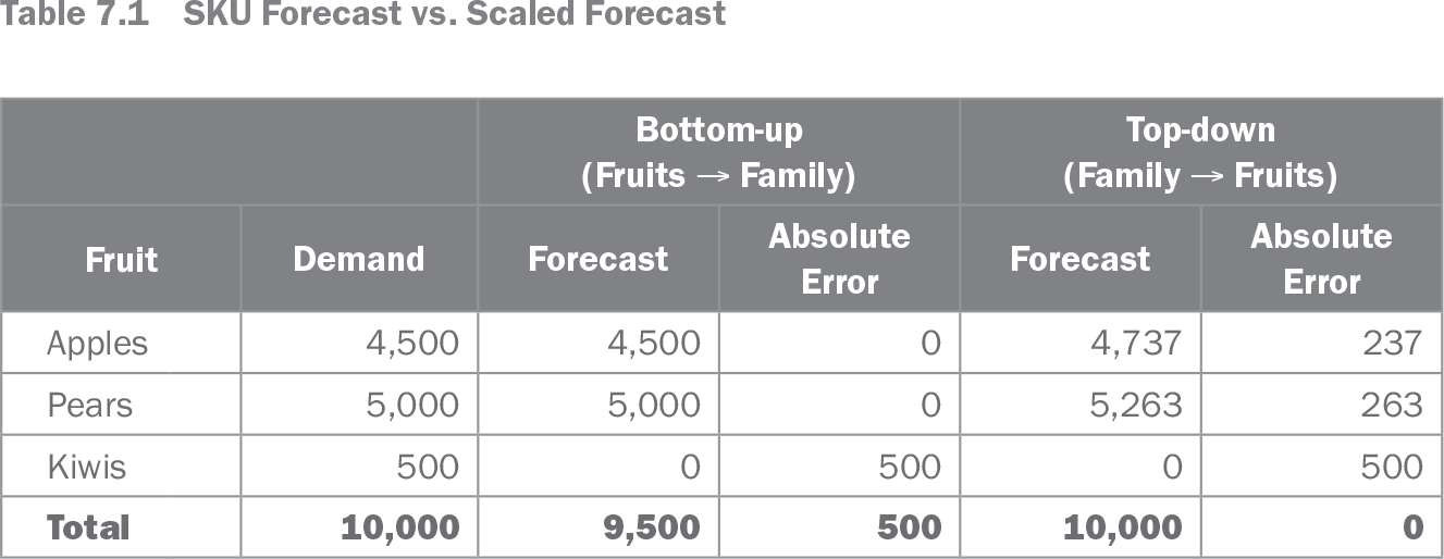
A supermarket forecasts 4,500 apples and 5,000 pears, producing a bottom-up family forecast of 9,500 fruits. A direct family forecast predicts 10,000. The family forecast is more accurate at the aggregate level, while the bottom-up forecasts are more accurate for apples and pears. The difference comes from sporadic kiwi sales that are difficult to predict at SKU level but visible in aggregate demand. Scaling the detailed forecasts to 10,000 would therefore reduce SKU-level accuracy. section 7.3.3
Do not assume that detailed forecasts will match a direct aggregate forecast. The forecast of a sum is not necessarily the sum of forecasts. Product introductions, end-of-life items, substitutions, shared demand drivers, and sporadic sales can make long-term bottom-up forecasts unsuitable for a stable product-family total. section 7.3 section 7.3.2
Table 7.1 SKU Forecast vs. Scaled Forecast (view table figure)
| Bottom-up (Fruits → Family) |
Top-down (Family → Fruits) |
||||
|---|---|---|---|---|---|
| Fruit |
Demand |
Forecast |
Absolute Error |
Forecast |
Absolute Error |
| Apples |
4,500 |
4,500 |
0 |
4,737 |
237 |
| Pears |
5,000 |
5,000 |
0 |
5,263 |
263 |
| Kiwis |
500 |
0 |
500 |
0 |
500 |
| Total |
10,000 |
9,500 |
500 |
10,000 |
0 |
Inspect the fruit example’s SKU-level and family-level errors to compare where bottom-up and top-down forecasts create value. section 7.3.3