Top-down forecasting starts with demand at an aggregate level, then disaggregates it into products, stores, days, or stock keeping units. It helps planners choose a forecast granularity that supports sourcing, production, and delivery decisions. section 5.2 section 5.4
Use top-down forecasting by:
- Forecasting a family total, such as all ice creams, instead of forecasting each flavor independently when substitution or cannibalization obscures SKU demand. section 3.3
- Splitting a high-level forecast with a flat allocation or historical weighted averages, such as distributing national demand among stores by historical revenue. section 5.2
- Selecting the aggregation level according to decision usefulness, data availability, materiality, geography, and time horizon rather than defaulting to SKU-level forecasts. section 5.4
Fruit demand at a supermarket
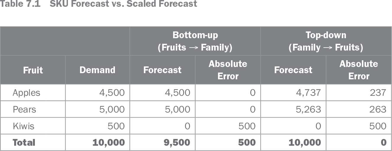
A supermarket expects monthly demand for 10,000 fruits. A bottom-up forecast predicts 4,500 apples, 5,000 pears, and no kiwis, totaling 9,500. A top-down family forecast predicts 10,000 fruits and allocates 4,737 apples, 5,263 pears, and 0 kiwis. The family forecast captures sporadic kiwi demand and is more accurate at family level, while the bottom-up forecast is more accurate for apples and pears. Scaling the bottom-up result to 10,000 does not improve SKU accuracy. section 7.3.3
Table 7.1 SKU Forecast vs. Scaled Forecast (view table figure)
| Bottom-up (Fruits → Family) |
Top-down (Family → Fruits) |
||||
|---|---|---|---|---|---|
| Fruit |
Demand |
Forecast |
Absolute Error |
Forecast |
Absolute Error |
| Apples |
4,500 |
4,500 |
0 |
4,737 |
237 |
| Pears |
5,000 |
5,000 |
0 |
5,263 |
263 |
| Kiwis |
500 |
0 |
500 |
0 |
500 |
| Total |
10,000 |
9,500 |
500 |
10,000 |
0 |
Compare bottom-up and top-down forecasts, allocations, and absolute errors across fruit SKUs and the family total. section 7.3.3
Top-down forecasting is not a universal solution. Family definitions may be debatable, recent stockouts can distort allocation ratios, and stable family totals may still be difficult to translate into future SKU composition. Product life cycles can make long-term SKU disaggregation especially uncertain. section 3.3 section 7.3.2