A contact map records which parts of a biomolecule are spatially close. For a protein of length L, a residue contact map is an L × L binary matrix: entry C[i, j] is 1 when residues i and j are in contact and 0 otherwise. It compresses information about the folded protein into a form suitable for computation. section 11.3.1
One contact definition measures the distance between residues’ C-beta atoms, using C-alpha for glycine, and marks pairs within 8 angstroms. This empirically chosen cutoff captures potentially interacting residues without making the map overly dense. A contact indicates proximity, not proof of a specific interaction. Rotating or moving the protein does not change its contact map. section 11.3.1
Figure 11.5 Transforming a Protein's 3D Structure into a 2D Graph. Converting a protein's spatial information into a graph representation. (a) A simplified 3D protein structure with dashed lines connecting amino acid residues that are in close spatial proximity (a 'contact'). (b) Spatial information is translated into a contact map, which is a 2D matrix. A point at (i, j) is marked if residue i and residue j are in contact, serving as an adjacency matrix for the graph. (c) The contact map is used to construct a graph where the amino acid residues are the nodes and the contacts are the edges. This graph captures the key residue interactions in a format that is invariant to the protein's rotation and translation in 3D space.
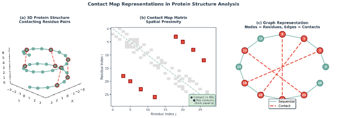
Follow the conversion from a folded protein to a contact matrix and then to a residue graph. section 11.3.1
The contact matrix can serve as a graph’s adjacency matrix: residues become nodes, and contacts become edges. A graph neural network can use this representation when predicting drug–target affinity, alongside features describing each residue. section 11.3.1 section 11.3
Listing 11.3 Construct Protein Graph from Contact Map and Sequence
def target_to_graph(target_key, target_sequence, contact_dir, aln_dir):
    target_size = len(target_sequence)
    contact_file = os.path.join(contact_dir, target_key + '.npy')
    contact_map = np.load(contact_file)
    assert contact_map.shape[0] == target_size
    contact_map += np.eye(    #A
        contact_map.shape[0]    #A
    )    #A

    threshold = CONFIG['contact_map_threshold']    #B
    index_row, index_col = np.where(contact_map >= threshold)
    target_edge_index = []
    for i, j in zip(index_row, index_col):
        target_edge_index.append([i, j])

    aln_file = os.path.join(aln_dir, target_key + '.aln')
    target_feature = compute_target_feature(    #C
        aln_file, target_sequence    #C
    )   #C
    target_edge_index = np.array(    #C
        target_edge_index    #C
    )    #D

    return target_size, target_feature, target_edge_index
The graph-construction listing loads a contact map, adds self-connections, and selects entries at or above a configured threshold as edges; it also computes residue features. section 11.3.1
A map can be derived by thresholding distances in an experimental or predicted structure. When a structure is unavailable, a contact predictor can instead use sequence information. Multiple sequence alignments collect related sequences, where correlated mutations can provide evidence of spatial contacts; Pconsc4 uses this evolutionary signal to predict a map. section 11.3 section 11.3.1 section 11.8
Predicted maps are imperfect. Experimental structures also capture particular conformations and conditions and may omit flexible or ligand-dependent regions. The representation therefore trades structural detail against the availability and quality of its input data. section 11.3 section 11.8
Contacts in protein language models
Some ESM-2 attention heads track residues that are far apart in sequence but close in the folded protein. Logistic regression on these attention maps can recover a contact map reasonably well, suggesting that sequence-trained representations contain structural information. section 12.3.5
