Contact prediction infers which residue pairs are spatially close from protein sequence information, enabling graph construction when experimental structures are unavailable. section 11.3.1
A practical contact-prediction workflow:
- Collect homologous protein sequences and align them in a multiple sequence alignment (MSA). section 11.3.1
- Detect correlated mutations, using compensatory evolutionary changes as evidence that residues interact physically. section 11.3.1
- Use a deep-learning model trained on known Protein Data Bank structures to predict a contact map. section 11.3.1
From contact map to protein graph
A graph-building pipeline loads a predicted contact map, thresholds its entries into residue-to-residue edges, computes sequence-derived features from an alignment, and represents residues as graph nodes. section 11.3.1
Figure 11.5 Transforming a Protein's 3D Structure into a 2D Graph. Converting a protein's spatial information into a graph representation. (a) A simplified 3D protein structure with dashed lines connecting amino acid residues that are in close spatial proximity (a 'contact'). (b) Spatial information is translated into a contact map, which is a 2D matrix. A point at (i, j) is marked if residue i and residue j are in contact, serving as an adjacency matrix for the graph. (c) The contact map is used to construct a graph where the amino acid residues are the nodes and the contacts are the edges. This graph captures the key residue interactions in a format that is invariant to the protein's rotation and translation in 3D space.
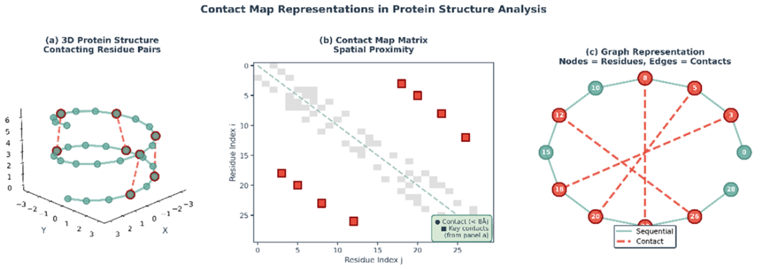
Trace how three-dimensional residue proximity becomes a two-dimensional contact map and then a rotation- and translation-invariant protein graph. section 11.3.1
