A continuous distribution represents uncertainty about a quantity whose possible values form a continuous range. For example, a tea preference rate can be 0.63432 or 0.34269 rather than only a rounded set of values. This avoids the approximation and precision problems caused by discretizing the range. section 3.0 section 3.1
The key ideas are:
- A probability density function describes how probability is distributed across a range; its height is not the probability of one exact value. section 3.2
- Integrating the density over an interval gives the probability that the quantity falls within that interval. section 3.2 section 3.3
- A single exact value has probability effectively zero, because it occupies no width; meaningful questions use ranges such as 0.1 to 0.2. section 3.3
Uniform uncertainty about a preference rate
Suppose every value of p from 0 to 1 is equally plausible. A uniform continuous distribution assigns equal density throughout that interval. The probability that p lies between 0.1 and 0.2 is 10%, while the probability that p is at least 0.5 is 50%. These probabilities come from the areas under the density curve, not from its height at an individual point. section 3.2 section 3.3
Figure 3.1 The procedure of deriving the posterior distribution under a Bayesian model: the prior is multiplied with the likelihood to produce the unnormalized posterior probabilities. These values are then normalized so that they sum to 1 to yield the posterior probabilities.
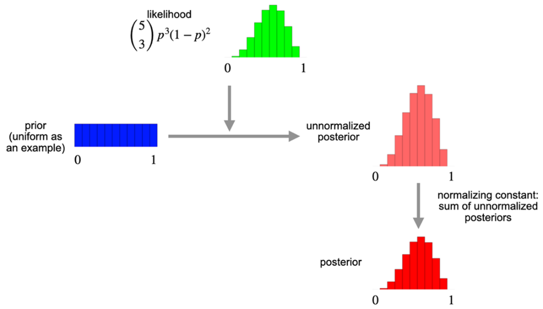
Trace how a Bayesian prior and likelihood combine into an unnormalized posterior, then normalize the result to represent updated belief. section 3.1