A continuous distribution models a quantity that can fall anywhere along a range, such as adult height, time between views, coffee weight, or dog weight. Measurements may be recorded in whole units, but the underlying quantity can still vary between those recorded values. section 3.12 section 4.3 section 4.5
Unlike a discrete distribution’s separate bars, a continuous distribution is usually drawn as a smooth curve. The curve’s vertical value is probability density, not the probability of one exact value. Probability comes from an area under the curve, and the total area is 1.0. section 3.8 section 4.5
Figure 3.6 The beta distribution showing probabilities of success rates for a single trial
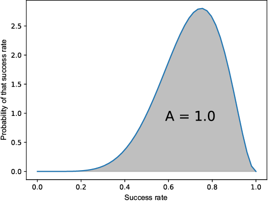
A beta curve makes the distinction visible: its height shows density across possible success rates, while its full area represents total probability. section 3.8
For a range, calculate the area between its endpoints. A cumulative distribution function (CDF) gives the area to the left of a value, so subtracting two CDF results gives the probability between them. For a beta distribution with 7 successes and 3 failures, the area from 0.4 to 0.7 is about 0.4378. section 3.8
A range beats an exact weight
If golden retriever weights follow a normal distribution with mean 64 pounds and standard deviation 3 pounds, the probability of exactly 61.63 pounds is 0. Instead, ask for a useful interval: the probability from 61 to 63 pounds is about 0.2108. section 4.5
Continuous models can generalize measured data. Coffee-ground responses recorded as whole grams can be treated as values on a continuous scale; a normal distribution uses the mean and standard deviation to set the curve’s location and shape. section 4.3

