Convolution

As explained in Graph Neural Networks in Action

Convolution is an operation that combines nearby values through a local filter or weighted aggregation to produce a transformed representation.

Convolution combines nearby values through a local filter or aggregation to produce a representation that makes downstream tasks easier. In images, the filter moves across a fixed pixel grid; in graphs, convolution operates across neighborhoods of nodes. section 3.4.1 section 3.0

A practical convolutional layer can be understood as a short pipeline:

• Apply a learnable filter or kernel to highlight features in the input. section 3.4.1
• Pass the filter output through an activation function for a nonlinear transformation. section 3.4.1
• Optionally pool the result to reduce its size for subsequent learning tasks. section 3.4.1
• Choose a spatial method that slides a filter across graph structure, or a spectral method that filters graph signals. section 3.4.1

Figure 3.11 A convolution of an input image (left). The kernel (middle) is passed over the image of an animal, resulting in a distinct representation (right) of the input image. In a deep learning process, the parameters of the filter (the numbers in the matrix) are learned parameters.

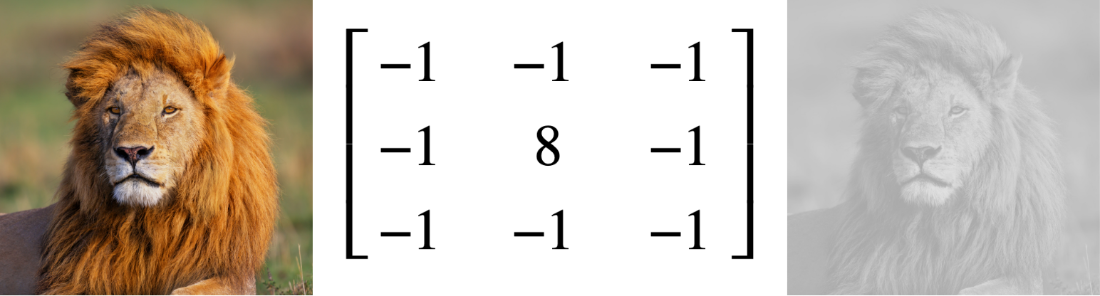
Use the image-and-kernel visualization to see how learned filter weights produce a distinct transformed representation. section 3.4.1

Figure 3.12 A comparison of convolution over grid data (left; e.g., a 2D image) and over a graph (right).

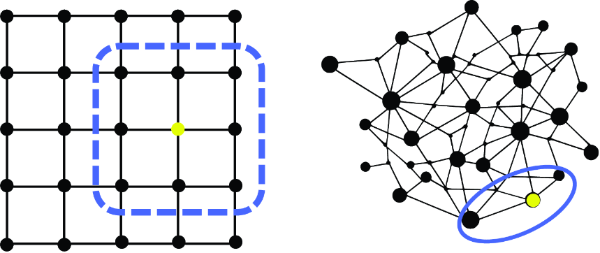
Use the grid-versus-graph comparison to connect pixel neighborhoods with graph neighborhoods. section 3.4.1

How Graph Neural Networks in Action covers it

How deep it goes

Defines filters, activations, pooling, spatial methods, and spectral methods without deriving the mathematical convolution operator.

Examples

Uses image kernels, pixel grids, graph neighborhoods, graph signals, and node prediction as concrete examples.

What it assumes

Assumes graph and graph representation learning foundations while providing a short primer on convolution.

What you can do after

Apply convolutional GNNs to node prediction and interpret them as neighborhood-based representation learners.

How it connects

Links convolution to convolutional neural networks, graph convolutional networks, GraphSAGE, graph signals, and message passing.

liveBookmanning.com

Read Graph Neural Networks in Action on liveBook Get the book at manning.com

Related concepts

• convolutional neural networkused by · A convolutional neural network is a neural-network architecture that applies learned convolutional operations to extract patterns from structured data.
• sliding windowuses · A sliding window is a bounded region over an ordered sequence or time range that advances, updating which elements fall within it.
• inner productuses · An inner product is a scalar-valued operation on two vectors that combines their corresponding components, summing their products and, for complex vectors, using conjugation.
• dilated convolutionincludes · A dilated convolution applies a filter whose sampling positions are spaced apart, expanding the receptive field without proportionally increasing kernel size or parameters.
• strided convolutionincludes · A strided convolution is a convolution whose filter moves across input positions by more than one step, typically reducing spatial or temporal resolution.

This explainer was generated by Manning's knowledge graph from the text of Graph Neural Networks in Action. The section links point to the parts of the book it draws on.