DBSCAN

As explained in Advanced Algorithms and Data Structures

DBSCAN is a density-based clustering algorithm that identifies dense regions and separates them from lower-density points using neighborhood and density parameters.

Suppose customer data contains groups with irregular boundaries, plus a few customers unlike any group. DBSCAN clusters points by local density rather than by distance to a centroid. It does not require a preset number of clusters: each point belongs to at most one cluster, or is marked as noise. section 12.0 section 12.3

Choose a neighborhood radius ε and a minimum count minPoints, then classify points by their neighborhoods:

• A core point has at least minPoints points, including itself, within ε. section 12.3.1
• A point within ε of a core point is directly reachable from it. A chain of core points can make more distant points density-reachable; its final point need not be core. section 12.3.1
• Reachable core points grow the same cluster. A non-core point reached from a core point can join that cluster without extending it. Points unreachable from any core point are noise. section 12.3.1 section 12.3.2

To build a cluster, start at an unassigned point and keep a set of points to process. Query each point’s ε-neighborhood. If it is a core point, add its undiscovered neighbors to the cluster and processing set; otherwise, do not expand from it. Finish that cluster before starting another. Each point goes through the main loop once, rather than repeatedly adjusting centroids as in k-means. A border point reachable from two clusters may join whichever is processed first, so the result is not entirely independent of processing order. section 12.3.2 section 12.3

Figure 12.10 A few steps of the main loop of DBSCAN. When core points are processed (the first three steps in the figure) all their undiscovered neighbors are added to current cluster and to a set (not a queue) of points to be processed. Conversely, when the current point being processed is not a core point, like v in the last step, then no further action is taken.

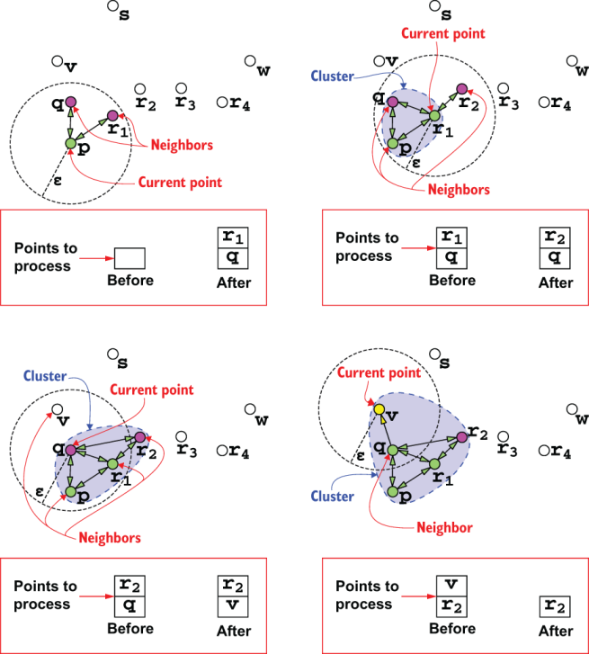
The step-by-step diagram shows why a core point adds neighbors to the current cluster, while processing a non-core point ends that branch of expansion. section 12.3.2

Neighborhood lookup dominates implementation choices. DBSCAN needs range queries for all points within ε, not nearest-centroid queries. A brute-force search across the dataset for each point gives O(n²) time. With a multidimensional index such as a k-d tree, the stated estimate is O(n log n) if each range query takes O(log n); range queries can still take O(n) in the worst case. section 12.3.3

Figure 12.13 Using the first example dataset in figure 12.12, we can see how sensitive to the choice of parameters (in particular of ϵ) the result of DBSCAN is. All the examples ran DBSCAN on the same dataset with parameter minPoints set to 3 (the dimension of the domain plus 1). (Left) Using a value too small for ϵ causes the dense area to be too small, so data is partitioned into too many small clusters. A few points, plotted with X-shaped markers, are even marked as outliers. (Center) When the right value for the domain is chosen, the result is that DBSCAN partitions data perfectly into two concentric rings. (Right) When the radius ϵ is set to a value so big that the dense area of inner points extends to points of the outer ring, then the whole dataset is mistakenly assigned to the same cluster.

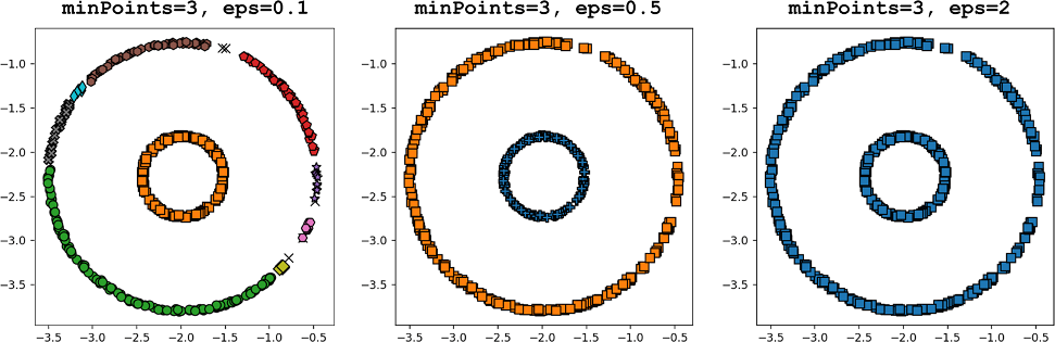
The concentric-ring example makes parameter tuning visible: an ε that is too small fragments clusters, while one that is too large merges the rings. section 12.3.4

DBSCAN can identify outliers and non-linearly separable, arbitrarily shaped clusters where k-means may fail. The trade-off is parameter sensitivity: regions with different densities may not admit one useful ε and minPoints setting. High-dimensional Euclidean distance can also become unhelpful, although other distance metrics are possible. For distributed data, sharding must preserve neighborhoods near boundaries; one MapReduce approach expands grid cells by ε, clusters each shard, then reconciles neighboring clusters. section 12.3.4 section 13.4

How Advanced Algorithms and Data Structures covers it

How deep it goes

Develops reachability definitions into a cluster-expansion algorithm, implementation, range-query costs, limitations, and a distributed variant.

Examples

Uses core-point diagrams, cluster-growth steps, concentric rings under different ε values, and expanded grid shards.

What it assumes

Assumes points and distance-based neighborhoods; defines core points and reachability before using them to construct clusters.

What you can do after

Build it from scratch using neighborhood queries and cluster expansion, then evaluate parameter and indexing trade-offs.

How it connects

Connects density-based clustering to k-means, range queries, k-d trees, OPTICS, and MapReduce.

liveBookmanning.com

Read Advanced Algorithms and Data Structures on liveBook Get the book at manning.com

Also explained in

• 

  liveBookmanning.com
  Data Without LabelsDBSCAN is a density-based clustering algorithm that identifies dense regions and labels sufficiently isolated points as noise.
• 

  liveBookmanning.com
  Outlier Detection in PythonDBSCAN is a density-based clustering algorithm that forms clusters from regions of sufficiently dense observations and can leave some observations unclustered.

Compare how 3 books explain DBSCAN →

Related concepts

• hard clusteringkind of · Hard clustering assigns each observation to at most one cluster, with all clusters represented at the same hierarchy level.
• clusteringkind of · Clustering is the technique of grouping data items according to similarity or shared characteristics.
• epsconfigured by · Eps is a numeric parameter or constant whose specific meaning depends on the method, often representing a tolerance, smoothing value, neighborhood radius, or floating-point precision.
• K-means clusteringcontrasts with · K-means clustering partitions data into a specified number of groups by assigning observations to representative centers and iteratively updating those centers to reduce within-group distances.
• core pointuses · A core point is a DBSCAN observation whose specified-radius neighborhood contains at least the required minimum number of observations, including itself.

This explainer was generated by Manning's knowledge graph from the text of Advanced Algorithms and Data Structures. The section links point to the parts of the book it draws on.