Degrees of freedom count the independent values available after constraints are accounted for. In these applications, the t-distribution uses degrees of freedom equal to the sample size minus one: n − 1. section 5.5 section 6.12
For samples of 30 or fewer, using the t-distribution instead of the normal distribution captures extra uncertainty through fatter tails. As degrees of freedom approach 30, the t-distribution converges toward the normal distribution. section 5.5 section 6.12
Use degrees of freedom to:
- Calculate a small-sample confidence interval with a t critical value and n − 1 degrees of freedom. section 5.5
- Run a small-sample hypothesis test by supplying n − 1 to the t-distribution functions. section 6.12
- Interpret smaller degrees of freedom as greater uncertainty rather than as evidence that a result is automatically unreliable. section 5.5
Ten candles, nine degrees of freedom
A candle maker measures the burn time of 10 candles. The calculation uses n = 10, so the t-distribution has 9 degrees of freedom. With a sample mean of 42.24, standard deviation of 3.62, and 99% confidence, Python calculates the interval using the t critical value for 9 degrees of freedom. section 5.5
Testing exam scores
A college samples 21 students, finding a mean of 110 against a claimed population mean of 100. The test uses 20 degrees of freedom, a right-tailed t-test, and significance level α = 0.01. section 6.12
Figure 5.8 The t-distribution with different degrees of freedom (DOF). Note that as the degrees of freedom approach 30, the distribution converges to a normal distribution.
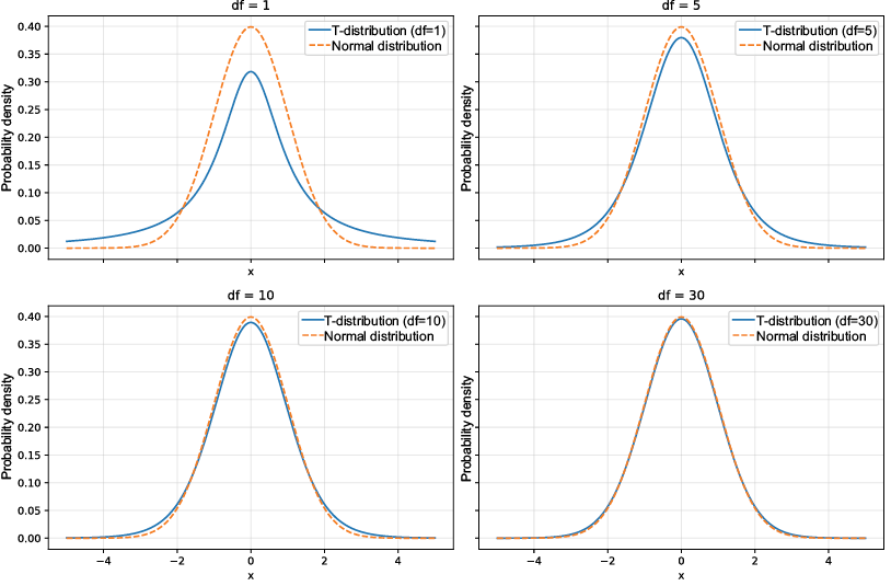
Compare t-distributions at different degrees of freedom and see their convergence toward the normal distribution. section 5.5


