For a unitary transformation \(U\), an eigenvector (or eigenstate) is a quantum state \(\ket{\psi}\) whose direction is unchanged by the operation: \(U\ket{\psi}=\lambda\ket{\psi}\). The scalar \(\lambda\) is its eigenvalue. Because a unitary preserves vector norm, \(|\lambda|=1\), so \(\lambda=e^{2\pi i\theta}\) for an eigenphase \(\theta\) between 0 and 1. The state may acquire a global phase, but otherwise remains the same physical state. section 5.3
Eigenvectors of the Z gate
The \(Z\) gate leaves \(\ket{0}\) unchanged, so \(Z\ket{0}=\ket{0}\): \(\ket{0}\) has eigenvalue \(1\) and eigenphase \(0\). It multiplies \(\ket{1}\) by \(-1\), so \(Z\ket{1}=-\ket{1}\): \(\ket{1}\) has eigenvalue \(-1\) and eigenphase \(0.5\). States differing only by a global phase, such as \(-\ket{0}\) or \(i\ket{1}\), represent the same eigenvector class. section 5.3
Figure 5.4 An eigenvector of a unitary is a vector that is multiplied by a scalar when this unitary is applied to it. This scalar is called the eigenvalue. An eigenvalue of a unitary can only be a complex number with absolute value 1, so it can be represented as an exponent using the real-valued eigenphase.
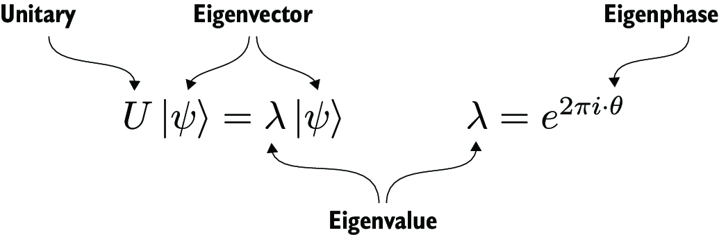
Use the diagram to connect the eigenvector equation with the unit-modulus eigenvalue and its real-valued eigenphase representation. section 5.3
Eigenvectors are useful when a circuit must expose a phase introduced by a gate. For controlled \(X\) and controlled \(-X\), \(\ket{+}\) and \(\ket{-}\) are eigenstates of the target operation. Their phase response can be transferred through phase kickback, while choosing control states that become orthogonal after the alternative operations enables single-experiment discrimination. More generally, states producing nearly orthogonal outputs are easier to distinguish, though repeated experiments and aggregated statistics may be needed. section 5.1.1
Quantum phase estimation treats the unitary and one of its eigenvectors as inputs:
- Prepare the supplied eigenvector and one or more auxiliary \(\ket{+}\) states. section 5.3.6
- Apply controlled versions of the unitary, then decode and measure the auxiliary qubits. section 5.3.6
- Return a classical estimate of the eigenphase associated with that eigenvector. section 5.3.6
- Test several unitary–eigenvector pairs against mathematically calculated phases, including \(Z\), \(INC\), and \(T\). section 5.3.6
A two-bit Qiskit implementation accepts the eigenvector as an amplitude list and uses `initialize` to prepare it. A Q# implementation instead accepts an eigenstate-preparation operation, allowing simple states to be prepared directly and more involved states through a library operation. Both approaches apply controlled unitaries and read out a classical phase estimate; test code can separately verify that each preparation really is an eigenstate of its unitary. section 5.3.6 section 5.3.7