Empirical rule

As explained in Grokking Statistics

A rule stating that approximately 68%, 95%, and 99.7% of observations from a normal distribution lie within one, two, and three standard deviations of the mean, respectively.

The empirical rule quickly estimates what is typical or extreme when data follows a normal, bell-shaped distribution. Starting with the mean, count outward in standard deviations. section 4.7

For normally distributed data, the approximate coverage is:

• About 68% lies within 1 standard deviation of the mean. section 4.7
• About 95% lies within 2 standard deviations of the mean. section 4.7
• About 99.7% lies within 3 standard deviations of the mean. section 4.7

A perfect coffee measurement

Suppose the mean measurement is 27.6 grams and the standard deviation is 3.2 grams. The rule gives ranges of 24.4–30.8 grams for 68%, 21.2–34.0 grams for 95%, and 18.0–37.2 grams for 99.7%. These are estimates only when the measurements follow a normal distribution. section 4.7

Figure 4.10 The empirical rule of the standard deviation

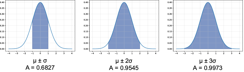
Use the normal-curve figure to see how expanding one, two, and three standard deviations captures increasingly large areas. section 4.7

mu, sigma = 27.6, 3.2

min68, max68 = mu-sigma*1, mu+sigma*1
print(f"68% of baristas report coffee measurement between {min68:.1f} and {max68:.1f} grams")

min95, max95 = mu-sigma*2, mu+sigma*2
print(f"95% of baristas report coffee measurement between {min95:.1f} and {max95:.1f} grams")

min99_7, max99_7  = mu-sigma*3, mu+sigma*3
print(f"99.7% of baristas report coffee measurement between {min99_7:.1f} and {max99_7:.1f} grams")

# 68% of baristas report coffee measurement between 24.4 and 30.8 grams
# 95% of baristas report coffee measurement between 21.2 and 34.0 grams
# 99.7% of baristas report coffee measurement between 18.0 and 37.2 grams

Use the Python listing to calculate the three ranges from a mean and standard deviation. section 4.7

How Grokking Statistics covers it

How deep it goes

Defines three coverage levels and works through numeric ranges, but stops short of formal derivation.

Examples

Applies the rule to baristas’ reported coffee measurements using a mean of 27.6 grams and standard deviation of 3.2 grams.

What it assumes

Assumes a normal distribution and known mean and standard deviation; introduces the coverage rule through a concrete example.

What you can do after

Apply it via simple arithmetic or Python to estimate ranges containing 68%, 95%, or 99.7% of normally distributed observations.

How it connects

Connects the normal distribution, mean, standard deviation, cumulative distribution functions, and central limit theorem.

liveBookmanning.com

Read Grokking Statistics on liveBook Get the book at manning.com

Related concepts

• standard deviationuses · Standard deviation is the nonnegative square root of variance and measures the typical dispersion of values around their mean in the original units.
• anomalyuses · An anomaly is an observation, behavior, or state that deviates from an expected or typical pattern or condition.
• normal distributionuses · A normal distribution is a continuous probability distribution with a symmetric, bell-shaped density determined by its mean and variance.

This explainer was generated by Manning's knowledge graph from the text of Grokking Statistics. The section links point to the parts of the book it draws on.