Suppose you need to find an unknown number. Knowing that it could be any of 100 numbers feels less certain than knowing it must be one of two. Entropy puts a number on that uncertainty using the probabilities of the possibilities, rather than how far apart their numerical labels are. section 13.3 section 13.7
For a discrete distribution with probabilities p₁ through pₙ, entropy is H = −Σ pᵢ log₂(pᵢ). In words, take the logarithm of each probability, weight it by that probability, add the results, and negate the sum. Using base 2 gives entropy in bits. Entropy is highest when the outcomes are equally likely; it falls as probability concentrates and reaches zero when one outcome is certain. section 13.4
Figure 13.4 Entropy is maximized under a uniform distribution. As the distribution becomes more peaked, entropy approaches 0, which happens when all probability is assigned to one single outcome.
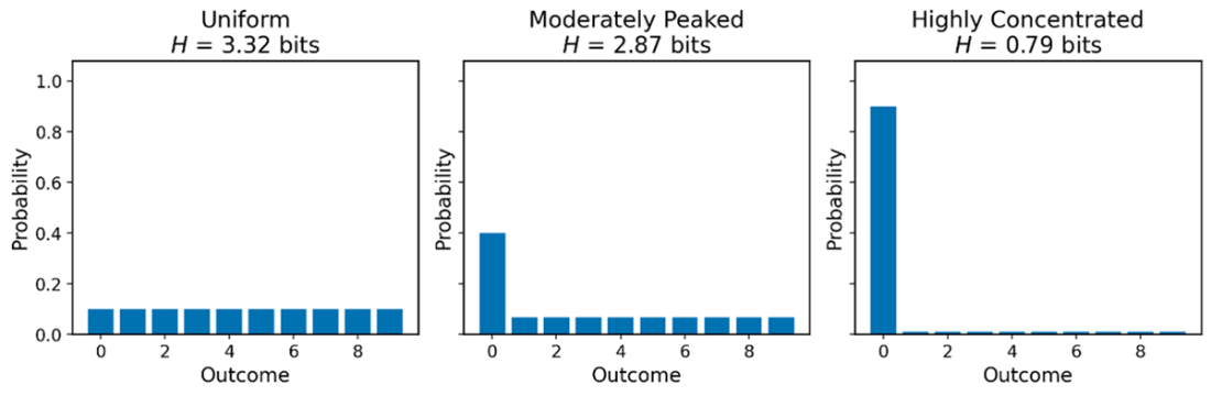
Compare the uniform, moderately peaked, and highly concentrated distributions to see how entropy changes as probabilities shift. section 13.4
Choosing a useful question
Give each integer from 1 to 100 equal prior probability. Its entropy is about 6.64 bits. Ask, “Is the number greater than 50?” Either answer leaves 50 equally likely possibilities, with entropy about 5.64 bits. The expected reduction is therefore 1 bit. A less balanced split leaves higher expected posterior entropy, making it a less informative question. For N equally likely states, the calculation simplifies to H = log₂(N); Python’s math.log2(N) implements that shortcut. section 13.7
This difference between entropy before an observation and expected entropy afterward is expected information gain (EIG). It lets you compare questions or experiments before collecting data: consider their possible outcomes, calculate the resulting posterior entropy for each, then average across outcomes. When that requires many expensive posterior calculations, EIG can instead be expressed as mutual information and sometimes calculated more efficiently with a forward model. For continuous quantities, differential entropy plays a similar role, but its absolute value is less meaningful than differences used to measure information gain. section 13.10 section 13.11