Forecast error answers a practical question: by how much did a forecast differ from the demand that actually occurred? Measuring that gap is the starting point for assessing forecast quality, but the metric chosen can shape later decisions and create its own blind spots. No single indicator fits every demand-planning situation. section 8.0
For period t, compute forecast error as eₜ = fₜ − dₜ: forecast minus demand. A positive error means the forecast overshot demand; a negative error means it undershot demand. Keeping this sign matters because errors can later be averaged to reveal systematic over- or underforecasting. section 8.2
Four-period calculation
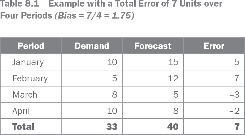
With demand and forecasts of 10 and 15 in January, the error is 5. February produces 7; March produces −3; and April produces −2. The total error is 7 units. Averaging those four errors gives a bias of 1.75, indicating an overall tendency to forecast above demand across the period. section 8.2 section 8.2
Table 8.1 Example with a Total Error of 7 Units over Four Periods (Bias = 7/4 = 1.75) (view table figure)
| Period |
Demand |
Forecast |
Error |
|---|---|---|---|
| January |
10 |
15 |
5 |
| February |
5 |
12 |
7 |
| March |
8 |
5 |
–3 |
| April |
10 |
8 |
–2 |
| Total |
33 |
40 |
7 |
Inspect the period-by-period demand, forecast, and signed error values before aggregating them into total error and bias. section 8.2
Compute errors over corresponding forecast horizons. For a Lag 1 forecast, compare the forecast made in one period with demand in the next period. In a spreadsheet, subtract demand from forecast for each row, then average the resulting error column for bias. When expressing bias as a percentage, divide average error by average demand from the same periods—not a wider date range. section 8.2.2
Use historical forecast error as evidence rather than as a universal score:
- Assess whether a forecast engine or process shows a consistent bias across multiple periods; a persistent pattern can signal that something is wrong. section 8.2
- Judge accuracy in context: forecastability changes with product granularity, time horizon, demand complexity, and industry conditions. section 10.0
- Classify products on the XYZ axis using relative historical forecast error, such as a combination of MAE% and Bias%, to identify items needing planner attention. section 13.2.2
- Avoid using demand variability or coefficient of variation as a substitute for forecastability; trend and seasonality can raise variability while remaining forecastable. section 13.2.2
A low or high error percentage is not self-explanatory. It is difficult to set a reasonable target without knowing the dataset: forecasting national monthly smartphone sales differs from forecasting a specific model in one store on one day. Review error alongside the decision context, then prioritize products where improving the forecast is likely to matter. section 10.0 section 13.4