Global-best particle swarm optimization (gbest PSO) uses a star-shaped neighborhood: every particle can access the best position found by the entire swarm. Each particle is therefore drawn toward the same shared result. This can speed convergence, especially on unimodal problems, but may leave too little exploration and trap the swarm in a local minimum. section 9.2.4
Figure 9.5 PSO neighborhood topologies: a) the star social structure, b) the ring topology, c) the Von Neumann model, and d) the wheel topology
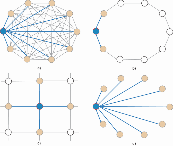
Compare the star's all-to-all communication with the more restricted ring, grid, and wheel neighborhoods. section 9.2.4
A practical implementation tracks both individual and shared progress:
- Give each particle a position, velocity, personal-best position, and personal-best objective value; track the swarm's global-best position separately. section 9.2.4
- Update velocity by combining its existing motion, attraction to the particle's personal best, and attraction to the global best. The parameters w, c1, and c2 weight these contributions. section 9.2.4
- Evaluate positions over repeated iterations and retain the best result found. Choose swarm size, iteration count, bounds, and velocity weights for the problem. section 9.2.4
Minimizing a two-dimensional function
For the Michalewicz function, one PySwarms setup uses 100 particles, two dimensions bounded from 0 to π, and 1,000 iterations. Its reported best position is approximately [2.203, 1.571], with an objective value of −1.8013. These are results of a run, not a guarantee that gbest PSO will find the optimum every time. section 9.2.4
!pip install pyswarms
import pyswarms as ps                                                      #1

dimension = 2                                                              #2
bounds = (np.zeros(dimension), np.pi * np.ones(dimension))                 #3

options = {'w': 0.9, 'c1': 0.5, 'c2': 0.3}                                 #4

optimizer = ps.single.GlobalBestPSO(n_particles=100, dimensions=dimension,
 options=options, bounds=bounds)                                         #5

cost, pos = optimizer.optimize(michalewicz_function, iters=1000)           #6

print(f"Optimal solution: {np.round(pos,3)}")                              #7
print(f"Minimum value: {np.round(cost,4)}")                                #7
#1 Import the PSO solver from pyswarms.
#2 Dimension of the Michalewicz function
#3 Create bounds for the search space.
#4 Set up the optimizer.
#5 Create an instance of the optimizer.
#6 Optimize the Michalewicz function
#7 Print the optimal solution and minimum value of the function after running PSO.
The PySwarms listing shows the objective, bounds, options, GlobalBestPSO constructor, and optimize call together. section 9.2.4
The same approach can search over continuous neural-network weights and biases. In a penguin-species classification comparison, global-best PSO reported 99.1% average accuracy, versus 69.1% for local-best and 43.8% for binary PSO. That comparison illustrates one application rather than a universal ranking: a ring-based local-best swarm converges more slowly but explores more of the search space and is recommended for multimodal problems. section 9.7 section 9.2.4
When experimenting, vary the problem features and PSO parameters, or try velocity clamping. Watch whether faster improvement comes at the cost of insufficient exploration. section 9.7 section 9.2.4
