When nearby points form a ring or another irregular shape, distance alone can suggest the wrong clusters. Spectral clustering instead represents points as graph nodes and uses their connections to find groups. The graph Laplacian is the matrix that carries those connections into the clustering calculation. section 5.3 section 5.3.1
In its simplest form, the Laplacian is L = D − A. D is the degree matrix: its diagonal records how many edges connect to each node. A is the adjacency matrix: its entries record which nodes are connected. Subtracting the matrices gives a representation that computers can use to analyze the graph. section 5.3.1
To use the Laplacian for spectral clustering:
- Build the adjacency and degree matrices from the connected data points, then calculate L = D − A. section 5.3.2
- Find the eigenvectors corresponding to the k smallest eigenvalues of L. Use the resulting matrix to cluster points in k-dimensional space. section 5.3.2
- For a two-cluster illustration, inspect the Fielder vector: its positive and negative components distinguish the two groups. section 5.3.2
Check a small graph by hand
In the illustrated graph, nodes 3 and 5 each have three connections, so their entries on D’s diagonal are 3; nodes with two connections have diagonal entries of 2. Construct A from the edges, subtract it from D, and compare your result with the illustrated Laplacian. The worked process then uses the Fielder vector’s signs to identify two clusters. For a Python implementation, use libraries rather than rebuilding every step from scratch. section 5.3.1 section 5.3.2
Figure 5.7 The Laplacian matrix is quite simple to understand. To get a Laplacian matrix, we can simply subtract an adjacency matrix from the degree matrix as shown in the example here. Here, D represents the degree matrix, A is the adjacency matrix, and L is the Laplacian matrix.
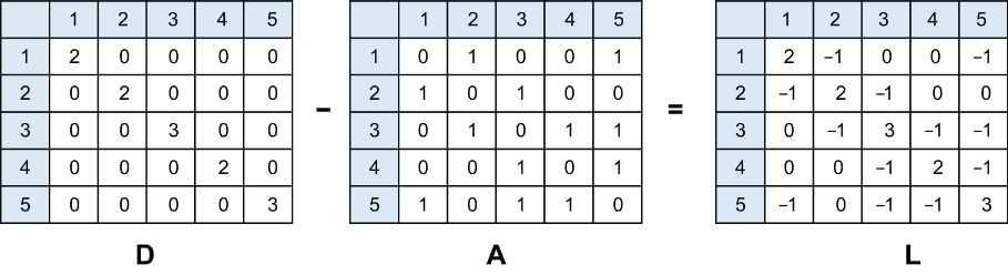
The matrix diagram shows the degree matrix minus the adjacency matrix, making the construction of L easy to check. section 5.3.1
