A degree matrix records how many connections each node has in a graph. It is a diagonal matrix: the entry for a node on the main diagonal is its number of incident edges, and every other entry is zero. This turns a simple connectivity count into a form that can be used alongside other graph matrices. section 5.3.1
Start with an adjacency matrix, whose rows and columns represent nodes and whose entries indicate whether two nodes are connected. Count each node’s connections and put that count in the matching diagonal position of the degree matrix, D. For the simplest graph Laplacian, subtract the adjacency matrix A: L = D − A. Spectral clustering then uses eigenvectors of L to represent and group connected data points. section 5.3.1 section 5.3.2
Check the connection counts
In a five-node example, nodes 3 and 5 each have three connections, so their diagonal entries are 3. The other nodes each have two connections, so their entries are 2. As a practice check, create D and A for a connected-point graph, calculate L = D − A, and compare the result with the supplied Laplacian. section 5.3.1 section 5.3.2
Figure 5.7 The Laplacian matrix is quite simple to understand. To get a Laplacian matrix, we can simply subtract an adjacency matrix from the degree matrix as shown in the example here. Here, D represents the degree matrix, A is the adjacency matrix, and L is the Laplacian matrix.
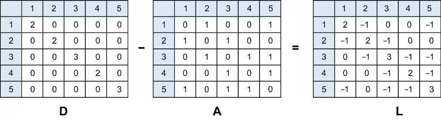
The diagram places the degree and adjacency matrices side by side and shows their subtraction to form the Laplacian. section 5.3.1
The matrix steps help explain spectral clustering, but a Python implementation can use existing libraries rather than build the algorithm from scratch. Connectivity-based clustering is useful when a shape such as two concentric circles makes distance-only grouping misleading. section 5.3.2 section 5.3
