Inverse distance interpolation estimates an unknown value as a normalized weighted sum of known values. Each weight is an inverse power of distance, so nearby points influence the result more strongly. section 8.3.1
For one variable, choose a power n and assign each known value yi the weight 1/|x−xi|^n. Increasing n makes the interpolant more local and produces more pronounced plateaus. At a known point, handle the zero distance explicitly and return its value. section 8.3.1 section 8.3.2
Extend the same idea spatially:
- In two dimensions, compute Euclidean distance from (x, y) to every known point and normalize the weighted sum. section 8.3.2
- In three or more dimensions, extend the distance formula and apply the same normalized weighting. section 8.3.2
- Use values or functions attached to the known points, depending on whether the interpolant represents samples or richer local behavior. section 8.3.1 section 8.3.2
A small terrain interpolator
Given xs = [2, 9, 8, 3, 5], ys = [1, 2, 9, 8, 5], and vs = [1, 2, 3, 4, 5], set n = 2. For each query (x, y), compute the distance to every sample, return the sample value on an exact match, otherwise accumulate vs[i]/distance^n and divide the weighted total by the weight total. This produces a surface suitable for procedural terrain. section 8.3.2
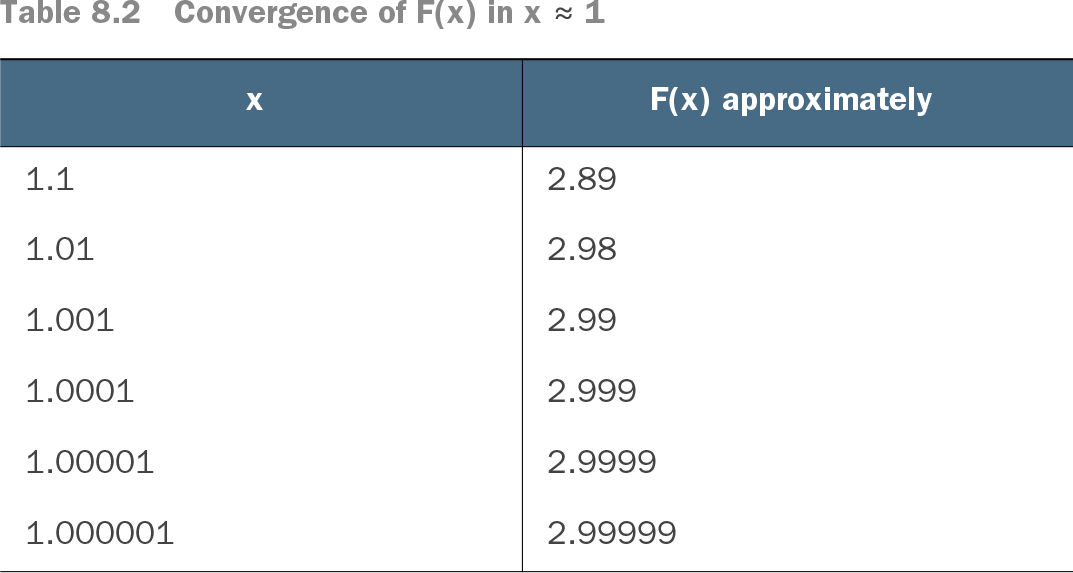
Table 8.2 Convergence of F(x) in x ≈ 1 (view table figure)
Compare values near a known point to see the interpolant converge toward that point’s value. section 8.3.1