A nonlinear classification problem may become linearly separable when observations are mapped into a richer feature space. But constructing every transformed coordinate can be impractical. A kernel function calculates the inner product in that space directly from the original observations: K(x, z) = ϕ(x) · ϕ(z), where ϕ is the feature transformation. This substitution is the kernel trick. section 8.6 section 8.6.1
In a support vector machine (SVM), the decision score can be written as f(x) = ∑ᵢ∈SV αᵢyᵢK(xᵢ, x) + b. Here xᵢ are support vectors, yᵢ their labels, αᵢ their fitted coefficients, and b the bias. The kernel supplies the transformed dot products; it does not replace the other components of the decision function. A hyperplane linear in the implicit feature space can correspond to a nonlinear boundary in the original space. section 8.6.1 section 8.6
The same dot product without transformed coordinates
Let ϕ(x) = (x, x²), so K(x, z) = xz + (xz)². For temperature readings 3 and 6, the transformed observations are (3, 9) and (6, 36), whose dot product is 18 + 324 = 342. The kernel gives K(3, 6) = 18 + 18² = 342 directly from the original readings. Both routes give the same value. section 8.6.1
Common kernels offer different ways to compare observations:
- Linear: K(x, z) = x · z. It uses the supplied feature space and produces a flat boundary in that space. section 8.6.2
- Polynomial: K(x, z) = (x · z + c)ᵈ. The degree d controls the powers and interactions represented, while c affects the influence of lower-degree terms. section 8.6.2
- Radial basis function (RBF): K(x, z) = exp(−γ||x − z||²). Gamma controls how locally the influence of a support vector is concentrated. section 8.6.2 section 8.6.3
Figure 8.7 The same synthetic two-class data fitted with linear, third-degree polynomial, and RBF kernels. The linear kernel produces a straight boundary, the polynomial kernel captures higher-order interactions through a curved boundary, and the RBF kernel produces a localized nonlinear boundary. The SVM framework remains unchanged; only the kernel used to compare observations differs.
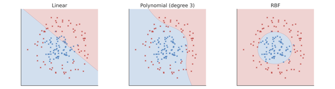
The same synthetic data produce a straight, curved, or localized boundary under linear, polynomial, and RBF kernels, respectively. section 8.6.2
A kernel defines a family of possible boundaries, not the fitted boundary by itself. Training data, support vectors, the soft-margin penalty C, and kernel parameters also matter. Higher polynomial degree or larger γ can capture more complex patterns but may fit training irregularities too closely. Evaluate candidate kernels and parameter combinations with cross-validation rather than training accuracy alone. Kernel SVMs can also become computationally expensive as the training set grows. section 8.6.2 section 8.6.3 section 8.8.2