A locally optimal solution is the best result an optimization process finds near its current position, not necessarily the best result overall. Imagine descending a mountain and stopping at a low point separated from a deeper valley by a rise. A loss-minimizing algorithm can likewise appear to converge at a local minimum while a lower value exists elsewhere. section 6.2.2
Figure 6.4 While the first figure is the point of convergence and represents the gradient descent method, note that in the second figure the global minima is somewhere else, while the algorithm can be stuck at a local minima. The algorithm might check that it has optimized the cost function and reached the point of global minima, whereas it has only reached the local minima. In a local minima, there is no direction that is ascending; all the directions descend. The algorithm, if purely local, has no information about other deeper minima existing beyond a potentially small hill.
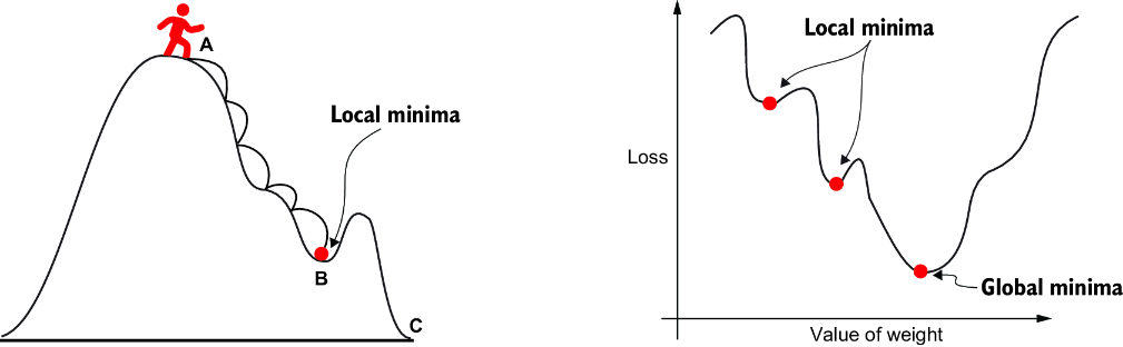
The two landscapes show why reaching a low point by following nearby changes does not establish that it is the global minimum. section 6.2.2
The distinction matters in several modeling workflows:
- In k-means, cluster assignments and centroids are updated until the clustering stops changing. Because the initial centroids are random, this is a local optimum; run the procedure multiple times and choose the best output. section 2.3.1
- In multidimensional scaling, gradient descent can settle at a local minimum of the loss function rather than the global minimum. A reported convergence point alone does not establish that the best possible solution was found. section 6.2.2
- In neural-network optimization, update behavior matters too: an overly large momentum update may pass over a local minimum, motivating the look-ahead approach of Nesterov accelerated gradient. section 8.2.6
Treat convergence as evidence that the current procedure has stopped improving, not as proof of global optimality. For k-means, compare results from repeated initializations rather than relying on a single run. section 2.3.1








