A Pareto chart combines descending bars with a cumulative-percentage line. Bars usually show frequencies, but they can show time, money, or another cost; the line tracks the running share of the total on a secondary y-axis. By putting the largest categories first, the chart makes nonlinear cause-and-effect patterns visible. section 15.4 section 20.5
Use a Pareto chart to ask a practical prioritization question: which relatively few causes account for the largest share of a problem or outcome? An 80–20 split is possible, not guaranteed. The useful finding may simply be that the relationship is nonlinear, helping focus corrective action where it can have the greatest effect. section 15.4 section 15.5
Read a Pareto chart in this order:
- Check that categories are sorted from the largest bar to the smallest; changing that order defeats the chart’s purpose. section 15.4
- Read each bar against the primary axis as that category’s frequency or cost. section 15.4
- Follow the aligned line point against the secondary axis to find the cumulative percentage after including that category. section 15.4
- Locate the categories needed to reach a decision-relevant cumulative share, such as 80%, then assess whether a small set dominates. section 15.4 section 15.5
NBA franchises: games played and won
For 47 active and inactive NBA franchises from 1946–2020, one chart uses games played as bars and cumulative total games as the line. A second uses games won. The results show nonlinearity rather than an 80–20 split: about 20% of franchises won roughly 45% of games, while roughly 42% of franchises accounted for 80% of wins. section 15.4.1 section 15.4.2
In R, ggplot2 plus ggQC can create a customizable chart with stat_pareto(), while qcc can create a chart and return a frequency and cumulative-percentage table. Prepare the categories first so labels remain properly sequenced; avoid broad binning when it would hide the individual results that matter. section 15.4.1 section 15.4.2
Figure 15.3 A Pareto chart built in ggplot2 and ggQC that displays the nonlinear relationship between NBA franchises and games played
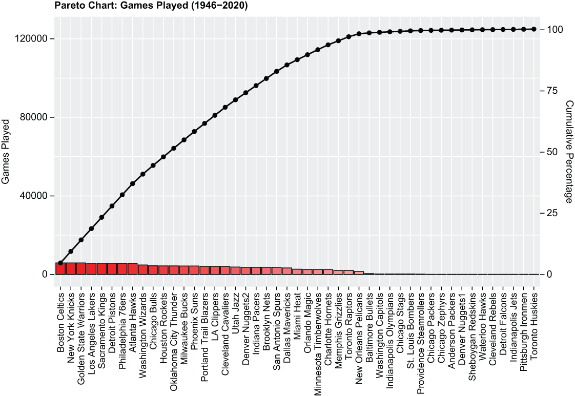
Inspect a franchise-level chart where descending game totals and the cumulative line reveal the nonlinear distribution without collapsing franchises into broad groups. section 15.4.1
