The Pearson correlation coefficient, written r, scores how closely two numerical variables follow a straight-line pattern. Think of temperature and sports drink sales: when warmer days generally mean higher sales, r is positive; when one rises as the other falls, r is negative. section 7.1 section 7.2
Its value runs from -1 to 1. Values near 1 indicate a tight upward linear relationship, values near -1 a tight downward one, and values near 0 little linear relationship. The coefficient is standardized covariance: how the variables move together relative to their variation. section 7.2
Figure 7.3 Different Pearson correlation values with different datasets. Note how a strong positive correlation (close to 1) or negative correlation (close to -1) has data that more closely resembles a line.
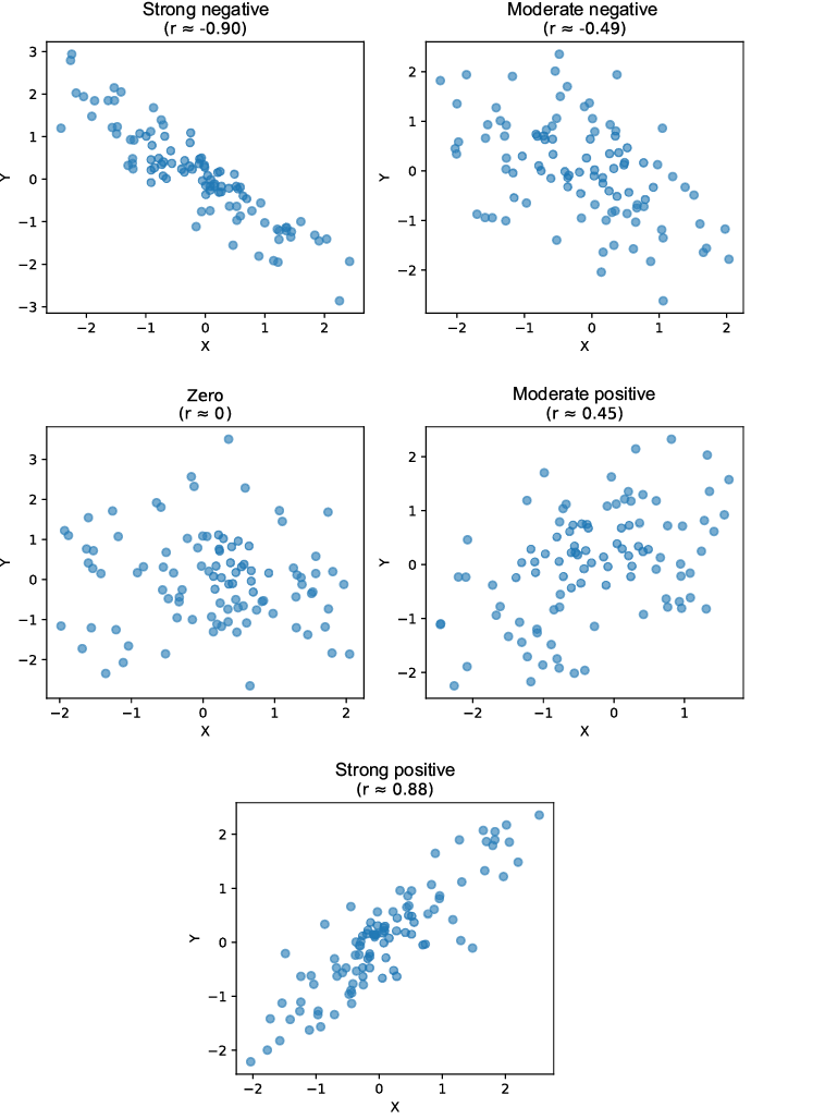
Compare the point clouds: stronger positive or negative correlations look more like a line, while weaker ones are more scattered. section 7.2
Temperature and sales
For 10 days of temperature and sports-drink sales, a manual calculation and SciPy's pearsonr both give r = 0.9889: a very strong positive linear association. That describes the observed pattern; it does not establish that temperature causes every change in sales. section 7.1 section 7.2 section 7.13
Use Pearson correlation carefully:
- Plot the data first. A coefficient can hide outliers, skew, or a pattern that is not adequately linear. section 7.12 section 7.13
- Check whether the data meet linear-analysis conditions, including homoscedasticity and no influential outliers. section 7.13
- Pair r with a p-value when testing whether a linear relationship is statistically significant, but do not treat either metric as automatic proof. section 7.0 section 7.13
- Do not turn association into causation or extrapolate the apparent trend beyond the observed data range. section 7.1 section 7.13
