Pose estimation predicts a body’s configuration. For motion prediction, the question is where its parts will move next given their recent positions. A walking foot, for example, moves in relation to the knee, leg, and rest of the body. That makes the task both relational and temporal: one still frame cannot show how those parts are moving. section 6.2 section 6.6
Represent each body joint as a graph node and each bodily connection between joints as an edge. At each timestep, node features can hold location and velocity. A sequence of these graphs preserves both the body’s structure and its changing position. section 6.2 section 6.3.1
One graph attention network (GAT) approach turns the sequence into a single spatiotemporal graph:
- Create a graph layer for each timestep, with edges between connected joints within that layer. section 6.3.1
- Connect corresponding joints across adjacent timesteps so information can travel through time. section 6.3.1
- Mask the nodes whose future features are unknown, then use earlier, unmasked nodes to predict them. section 6.3 section 6.3.1
Figure 6.9 Illustration of the spatiotemporal graph construction and inference process. Step 1 shows the sequence of graphs across timesteps with nodes representing entities at each timestep. Step 2 highlights intra-timestep edges (solid lines) connecting nodes within the same graph layer. Step 3 introduces inter-timestep edges (dotted lines) that encode temporal dependencies by linking corresponding nodes across adjacent timesteps. In Step 4, nodes at the final timestep are masked (gray) to represent unknown values for prediction. Step 5 demonstrates the inference process (dashed arrows), where information from unmasked nodes in earlier timesteps is used to estimate the features of masked nodes. The legend clarifies the types of nodes and edges used in the graph representation.
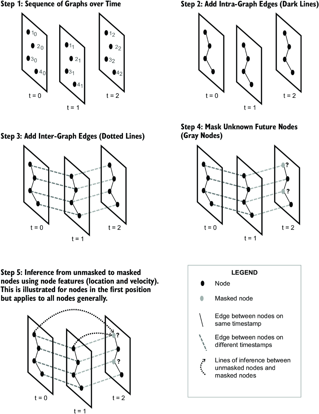
Follow the graph layers from within-frame connections through temporal connections to the masked future nodes; the diagram shows what information is available at prediction time. section 6.3.1
Predicting a walking subject’s next position
The CMU Motion Capture example tracks a walking subject with 41 sensors on joints from the toes to the neck. A PyTorch Geometric dataset combines their locations and velocities into node features and constructs edges across frames. The GAT is trained to predict masked features. This setup predicts a next step from recent motion; it does not by itself guarantee accuracy on entirely unseen kinds of data. An alternative encodes graph snapshots and models their evolution with recurrent networks and a variational autoencoder. section 6.2 section 6.3.1 section 6.0 section 6.3
