A posterior probability is an updated estimate made after evidence arrives. Start with a prior, observe an event, and use that information to calculate a more informed probability. section 8.2
Think of the three parts as a simple update:
- Prior: the initial probability before learning anything new. section 8.2
- Event: information that changes what you know. section 8.2
- Posterior: the final probability after incorporating the event. section 8.2
Spam email containing “lottery”
Suppose 20 emails contain the word “lottery”: 15 are spam and 5 are ham. The probability that an email is spam given this evidence is 15/20 = 0.75. Before seeing the word, the prior probability was 0.2; after seeing it, the posterior probability is 0.75. section 8.5
Bayes’ theorem formalizes this update from a prior and an event. With several events, naive Bayes combines them by assuming independence, which can produce useful approximations even when the assumption is imperfect. section 8.15 section 8.7
Figure 8.3 The prior, the event, and the posterior. The prior is the “raw” probability, namely, the probability we calculate when we know very little. The event is the information that we obtain, which will help us refine our calculation of the probability. The posterior is the “cooked” probability, or the much more accurate probability that we calculate when we have more information.
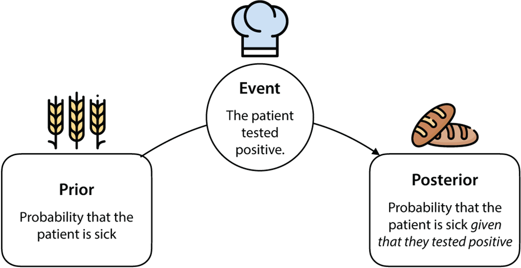
Use the prior–event–posterior diagram to visualize how evidence turns a rough probability into an updated estimate. section 8.2
model = {}
 for index, email in emails.iterrows():
    for word in email['words']:
        if word not in model:
            model[word] = {'spam': 1, 'ham': 1}
        if word in model:
            if email['spam']:
                model[word]['spam'] += 1
            else:
                model[word]['ham'] += 1
Inspect the small model-building function that counts word appearances in spam and ham emails before estimating posteriors. section 8.12