Prior probability

As explained in Grokking Machine Learning

A prior probability is the initial probability assigned to an event or hypothesis before new evidence is considered.

Will it rain today? Before you know where you are, you can make only a rough estimate. That initial estimate is a prior probability. Learning that you are in the Amazon rain forest gives you new information; the revised probability is called a posterior. section 8.1

A positive test does not tell the whole story

Suppose 100 of 1,000,000 people are sick. Before seeing a test result, the probability that a person is sick is 100/1,000,000, or 1 in 10,000. That is the prior. Even after a positive result, the chance of sickness is about 0.98% in this example: 99 sick people and 9,999 healthy people test positive. The starting frequency matters. section 8.1

Starting a spam filter

If 20 of 100 emails are spam, estimate P(spam) = 20/100 = 0.2 before inspecting a new email. This is the spam prior; the ham prior is 0.8. Among emails containing “lottery,” 15 are spam and 5 are ham, so the revised probability of spam for an email with that word is 15/20 = 0.75. section 8.2

Figure 8.5 We have removed (grayed out) the emails that don’t contain the word lottery. All of a sudden, our probabilities change. Among the emails that contain the word lottery, there are 15 spam emails and 5 ham emails, so the probability that an email containing the word lottery is spam, is 15/20 = 0.75.

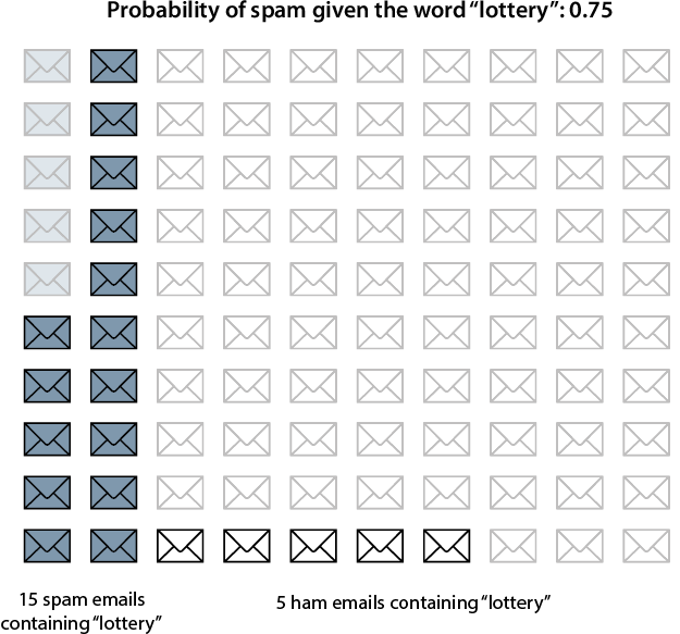
Filtering the email counts to messages containing “lottery” makes the change from the overall spam rate to the word-conditioned rate visible. section 8.2

To put a prior to work:

• Count the labeled cases in the class of interest and divide by the total. In a labeled email dataset, this gives a spam prior of about 0.24 and a ham prior of about 0.76. section 8.3
• Use evidence, such as words in an email, to revise the estimate. Naive Bayes combines a prior with several word events under an independence assumption; when a tested word is unknown to the model, its example prediction remains at the spam prior. section 8.3 section 8.4

Try counting spam and ham in a small labeled inbox. Calculate both priors, then pick a word and compare the overall spam rate with the spam rate among messages containing it. section 8.2

How Grokking Machine Learning covers it

How deep it goes

Defines the prior and calculates it from counts, then follows its revision through medical tests and email words.

Examples

Uses a rain forecast, medical-test counts, a 100-email spam example and a labeled email dataset.

What it assumes

Starts with counting and simple fractions, introducing prior and posterior probabilities in plain language.

What you can do after

Apply it via pandas to estimate spam and ham priors from labeled emails before making word-based predictions.

How it connects

Connects prior probability to Bayes’ theorem, posterior probability, conditional probability and naive Bayes.

liveBookmanning.com

Read Grokking Machine Learning on liveBook Get the book at manning.com

Also explained in

• 

  liveBookmanning.com
  Math and Architectures of Deep LearningThe distribution over parameters before observing data.
• 

  liveBookmanning.com
  Fabulous Adventures in Data Structures and AlgorithmsA prior is a probability distribution representing beliefs about a hypothesis before incorporating new evidence.
• 

  liveBookmanning.com
  Bayesian Optimization in ActionA prior distribution is a probability distribution representing beliefs about an unknown quantity before incorporating observations.
• 

  liveBookmanning.com
  AI-Powered SearchA prior distribution is a probability distribution representing an initial belief about an unknown quantity before incorporating case-specific observations.
• 

  liveBookmanning.com
  Build a Robo-Advisor with Python (From Scratch)A prior distribution is a probability distribution representing beliefs about an unknown quantity before incorporating observed data.
• 

  liveBookmanning.com
  Causal AIA prior distribution is a probability distribution expressing beliefs about unknown quantities before observing the relevant data.
• 

  liveBookmanning.com
  Machine Learning Algorithms in DepthA prior distribution represents probability beliefs about model parameters or latent variables before observing the current data.

Compare how 8 books explain prior probability →

Related concepts

• posterior probabilityproduces · A posterior probability or distribution expresses the probability assigned to an event, hypothesis, or unknown quantity conditional on observed evidence and prior information.
• bayesian statisticsused by · Bayesian statistics is a framework for statistical inference that combines prior probability distributions with observed-data likelihoods to update probabilities over hypotheses or unknown quantities.
• conjugacyincludes · Conjugacy is the property whereby a prior distribution and a specified likelihood yield a posterior distribution in the same family as the prior.
• probability distributionkind of · A probability distribution is a mathematical specification assigning probabilities to the possible values or outcomes of a random variable, with total probability one.
• Bayesian modelpart of · A Bayesian model represents uncertain quantities with prior distributions, likelihoods, and posterior distributions updated using observed data.

This explainer was generated by Manning's knowledge graph from the text of Grokking Machine Learning. The section links point to the parts of the book it draws on.