Pruning removes selected model components to reduce computational requirements or change behavior. A strategy decides what to remove, from individual neurons to entire Transformer blocks. More extensive removal can degrade capabilities and require recovery. section 1.2 section 1.2.1
Selection should follow the deployment objective. Domain data can identify components that contribute least to a target task; general structural importance metrics can guide efficiency-focused pruning without a domain dataset. Benchmark data can instead focus selection on a particular capability. section 1.2.5
Strategies differ in the components they remove:
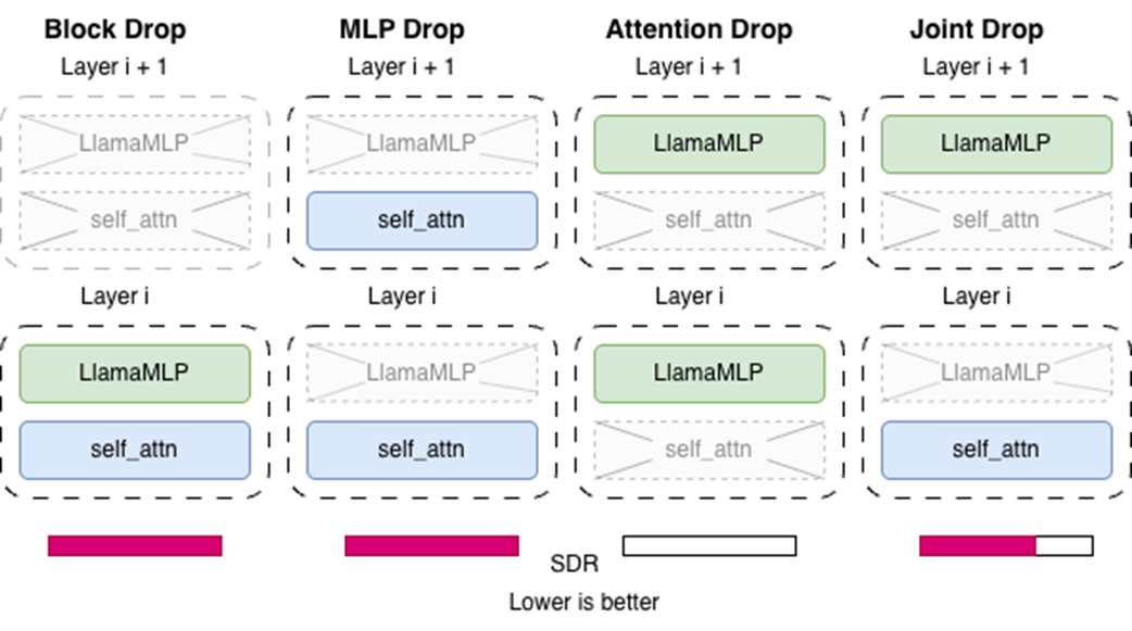
- Block Drop removes complete Transformer blocks, including attention and MLP. Cosine similarity between block input and output can identify candidates. section 8.5.1
- MLP Drop removes MLP layers; Attention Drop removes attention layers. Their effects can differ substantially within the same model. section 8.5.1
- Joint Layer Drop removes attention and MLP layers independently, rather than treating each block as indivisible. section 8.5.1
Figure 8.11 The four pruning strategies explored in He et al. (2024). Each column shows which modules are removed from a Transformer block (crossed out) and which are preserved. The bar at the bottom represents the SDR (Speedup Degradation Ratio). A shorter bar indicates a better trade-off between speed gain and quality loss. Attention Drop achieves the lowest SDR by a wide margin, making it the most efficient strategy despite leaving MLP layers intact.
Compare the components removed by each strategy and their speedup–degradation trade-offs. section 8.5.1
For depth pruning with optipfair, copy the teacher model, analyze layer importance on a data loader, sort scores, and remove the four lowest-scoring layers. Enable gradients on the remaining student parameters before recovery. section 6.1.3
Listing 6.5 Removing four less important layers
import optipfair as opf

student_model = deepcopy(teacher_model) #A
importance_scores = opf.analyze_layer_importance(student_model,
    train_dataloader,
    show_progress=True
) #B

LAYERS_TO_REMOVE = sorted(
    importance_scores.keys(),
    key=lambda x: importance_scores[x]
)[:4] #C

print (LAYERS_TO_REMOVE)
student_model = opf.prune_model_depth(
    model=student_model,
    layer_indices=LAYERS_TO_REMOVE,
    show_progress=True,
) #D

for param in student_model.parameters():
    param.requires_grad = True #E
The listing implements importance scoring, layer selection, pruning, and gradient enabling. section 6.1.3
Establish a baseline before pruning. Check generation quality, task-relevant benchmarks, model size, and inference time immediately afterward; then evaluate again after knowledge distillation. Perplexity can measure fluency for a generalist model, but a specialized system needs metrics aligned with its actual job. section 2.0 section 2.4 section 6.1.3
Compare removal and recovery
After four blocks were removed, the cosine-similarity candidate had perplexity 126 versus the teacher’s 13.38 and retained 78.6% of average benchmark capability. After distillation on 2,000 samples, its perplexity fell to 18.9 and retention rose to 86.7%. Other removal strategies degraded more initially but also recovered substantially. section 6.1.3
Measure the cost of a smaller model
Removing the final two layers of gemma-3-270m produced a model 4.16% smaller and 10% faster in the reported comparison, but most benchmark scores fell. A generation check also exposed factual errors and loss of focus before recovery. section 2.4
Speedup alone is not enough: the speedup degradation ratio divides percentage performance loss by percentage speedup, so a lower value indicates a better trade-off. Reported Attention Drop results had much lower ratios than Block Drop or MLP Drop, though results depend on the model and evaluation. section 8.5.1