Quadratic time complexity describes work that grows with the square of input size: for input length N, execution takes about N × N operations, or O(N²). Doubling N therefore multiplies the stated operation count by four. section 1.3.1
Look for this pattern when:
- Nested loops compare each element with every other element, as in bubble sort and insertion sort. section 1.3.1
- A larger input can demand much more computation; the practical impact depends on how large N becomes. section 2.1.3
From one ant to a full colony
One ant evaluating the remaining nodes at each tour step takes O(n²) operations. With m ants and I iterations, the total becomes O(I × m × n²): quadratic work per ant, repeated across the colony and iterations. section 8.1
Figure 1.1 List of categories of time complexity used in algorithm analysis, including constant time O(1), linear time O(N), quadratic time O(N^2), and logarithmic time O(logN). N represents the increasing input size, highlighting the performance differences in time complexities.
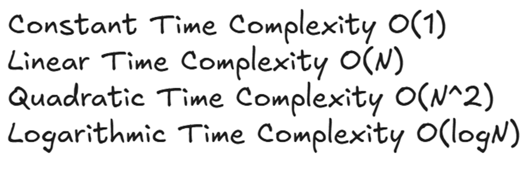
Compare quadratic growth with constant, linear, and logarithmic time as input size increases. section 1.3.1
Table 2.1 Time Complexity Analysis for N ranging from 10³ to 10⁶
|
N (Participants)
|
Performance
|
Time Complexity
|
|
N ≤ 10³ (1,000)
|
Instant response
|
O(10⁶)
|
|
N ≈ 10⁴ (10,000)
|
Fast (milliseconds)
|
O(10⁸)
|
|
N ≈ 10⁵ (100,000)
|
Borderline but with optimization feasible
|
O(10¹⁰)
|
|
N ≥ 10⁶ (1,000,000)
|
Impractical without heavy hardware modifications
|
O(10¹²)
|
See how the participant-count estimates move from instant response at 1,000 to impractical without heavy hardware modifications at 1,000,000. section 2.1.3