Quantum phase estimation (QPE) estimates the eigenphase φ of a unitary U when an associated eigenstate |ψ⟩ is available, with U|ψ⟩ = e^(2πiφ)|ψ⟩. The output is normally expressed as a binary fraction because applications need the real-valued phase rather than the complex eigenvalue. section 5.3
QPE treats the unitary and eigenstate as operations: prepare |ψ⟩, apply controlled forms of U, and measure a circuit designed to reveal a property of U. It is a reusable subroutine in Shor’s factoring algorithm, quantum counting, and HHL for linear systems. section 5.0 section 5.3
The key mechanism is phase kickback. Prepare each control qubit in |+⟩ and the target register in |ψ⟩. A controlled-U leaves the eigenstate unchanged while placing its eigenphase on the control register’s relative phases. Multiple control qubits provide multiple bits of requested precision. section 5.3.1 section 5.3.5
An inverse quantum Fourier transform then converts phase encoding into amplitude encoding. The computational-basis state representing the best binary approximation receives the largest amplitude; measuring the controls reads out the estimated binary fraction with high probability. section 5.3.5
A practical two-bit implementation follows this circuit workflow:
- Allocate two control qubits and an n-qubit target register; apply H to both controls and prepare the supplied eigenstate on the target. section 5.3.6
- Apply controlled-U operations so the controls acquire eigenphase information, then apply the inverse-QFT decoding gates. section 5.3.6 section 5.3.7
- Measure the controls, interpret the bit string as a binary fraction, and return the resulting classical eigenphase estimate. section 5.3.5 section 5.3.7
Testing with Z, INC, and T
Use known eigenvector–eigenphase pairs to test the circuit. For Z, |0⟩ has phase 0 and |1⟩ has phase 0.5; INC supplies phases 0, 0.5, 0.25, and 0.75; T on |1⟩ supplies phase 0.125. Run selected cases repeatedly and compare returned classical values with mathematically known phases. section 5.3 section 5.3.6 section 5.3.7
Figure 5.8 In quantum phase estimation algorithm, we use multiple control qubits to encode the information about the eigenphase in phases of their states. Then, we use inverse quantum Fourier transform to convert that information from phase encoding to amplitude encoding, increasing the amplitude of the basis state that encodes the eigenphase compared to the amplitudes of other states. Finally, we measure the control qubits, reading out the bits of the phase as measurement results with high probability.
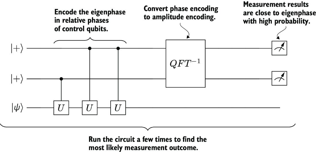
Inspect the QPE flow from phase kickback through inverse-QFT decoding to measurement. section 5.3.5