A random variable assigns a number to each possible outcome of a random experiment or process. It turns uncertainty into something that can be modeled: the number of absent employees, for example, can be assigned probabilities and used in a staffing decision. section 2.3 section 9.3
The possible values determine which kind of random variable you have:
- Discrete: distinct, countable values, such as the number of defects in a sample or the sum of two dice. Values between possible counts are not outcomes. section 2.4.1 section 2.4.2
- Continuous: values anywhere within a range, such as elapsed time or temperature. A displayed measurement may be rounded even when the quantity being modeled is continuous. section 2.3 section 2.3.1
For a discrete variable X, a probability mass function (PMF) gives the probability P(X = x) of each possible value. Its probabilities are nonnegative and sum to 1. For a continuous variable, a probability density function (PDF) describes how density varies across values; use it to reason about ranges rather than treating a plotted density as an individual outcome’s probability. A cumulative distribution function (CDF) gives F(x) = P(X ≤ x). section 2.4.2 section 2.3.2 section 2.4.3
Two dice: an outcome and a threshold
Let X be the sum of two six-sided dice. Among 36 equally likely rolls, one totals 2, two total 3, and three total 4. Thus P(X = 4) = 3/36, while P(X ≤ 4) = (1 + 2 + 3)/36 = 1/6, or about 16.7%. The first answers an exact-outcome question; the second answers a threshold question. section 2.4.2 section 2.4.3
Figure 2.4 The PMF for rolling a pair of six-sided dice, where the discrete random variable and its possible values, which are equal to the whole numbers between 2 and 12, are plotted along the x axis, and their respective probabilities of occurrence are plotted along the y axis. The y axis represents their actual probabilities, not their relative likelihood of occurrence. All probabilities are equal to or greater than zero.
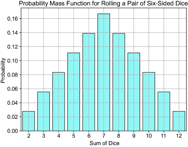
The two-dice PMF plots each possible sum against its probability, making the difference between a random variable’s values and their probabilities visible. section 2.4.2
Random variables also supply inputs to Monte Carlo simulations. For a call center, simulated counts of absent employees can help compare staffing outcomes when attendance varies. Check a process with known inputs before automating it: plausible-looking simulated results do not by themselves validate the model. section 9.0 section 9.3




