Regression to the mean is the pattern in which an extreme result is followed by a more moderate result, or by an opposite extreme that offsets it. In small or noisy groups, this can look like a meaningful rise or fall even when it is natural variation due to chance. section 8.5.1 section 16.3
The key practical question is whether a jagged pattern signals a real relationship or merely unstable observations. Results based on few records deserve particular caution: dramatic highs and lows may average out rather than support a decision rule. section 8.5.1 section 8.6
Shot-clock results for Milwaukee
For the 2019–20 Milwaukee Bucks, scoring and field-goal results at 19, 20, and 21 seconds alternated sharply around fitted trendlines. Strong performance with four seconds left offset weaker results one second earlier and later, illustrating why isolated extremes need not establish an optimal time to shoot. section 8.5.1 section 8.5.1
Figure 8.1 Average number of points scored (on the left) and field goal percentage (on the right) for the Milwaukee Bucks during the 2019-20 regular season computed at each second of a half-court possession, with trendlines
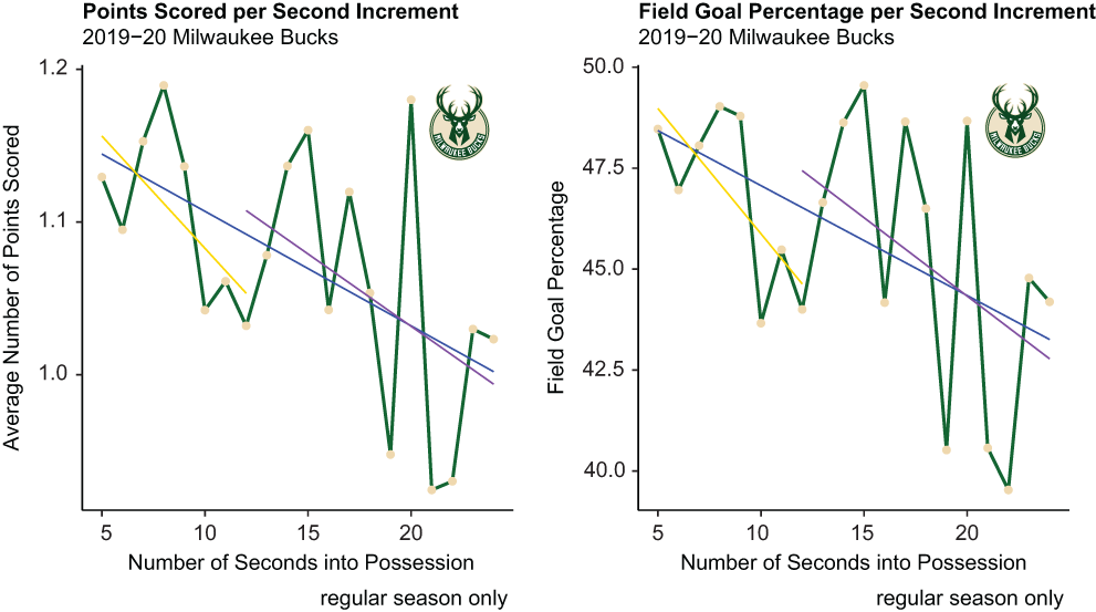
Compare the point and field-goal series with their trendlines to see how individual second-by-second values can sit far above or below an overall pattern. section 8.5.1
Aggregating all 30 NBA teams produces a much smoother series than examining one team at a time. The league-level plots show steep, similar downward trends as possessions run longer, so the earlier team-level swings no longer resemble regression to the mean or the letter of an optimal-stopping rule. section 8.5.4
Randomness is not a hot hand
A run of successes can tempt an analyst to infer that success causes more success. A fair-coin simulation instead models each flip as an independent trial with the same probability regardless of previous outcomes, helping separate random sequences from apparent order or causality. section 16.3
sample(x = c(0, 1), size = 10, prob = c(0.5, 0.5), replace = TRUE)
##  [1] 0 1 1 1 1 1 1 0 1 0
Run the fair-coin simulation to generate a short random sequence and inspect how streaks can occur without one flip changing the next flip’s probability. section 16.3
