A right-skewed, or positive-skewed, distribution clusters many observations at lower values and stretches into a long tail toward higher values. “Right” names the tail’s direction on the x-axis; “positive” names that same direction in numerical terms. section 2.5.3
A histogram makes this shape quick to spot. For NBA first-round selections from 2000–09, career win shares are right-skewed: many players accumulated few win shares, while a small number accumulated very large totals. section 2.5.3
p1 <- ggplot(draft, aes(x = WS)) +
 geom_histogram(fill = "royalblue3", color = "royalblue3",
                bins = 8) +
 labs(title = "Career Win Shares Distribution of
      NBA First-Round Selections",
      subtitle = "2000-09 NBA Drafts",
      x = "Career Win Shares",
      y = "Frequency") +
 theme(plot.title = element_text(face = "bold"))
print(p1)
Build an eight-bin ggplot2 histogram of career win shares, then inspect whether low-value bars dominate and a sparse tail extends rightward. section 2.5.3
Use the shape to turn a broad distribution into concrete follow-up questions:
- Check counts above a high threshold, such as 75 career win shares, to distinguish the small high-performing tail from the larger remainder. section 2.5.3
- Compare distributions across groups or years with boxplots, rather than assuming every draft class has the same spread of outcomes. section 2.5.3
- Read summary statistics alongside the chart: the example has a mean of about 29.35 win shares and a median of 19.6, with a maximum of 236.1. section 2.5.3
For a continuous probability distribution, right skew can be described as a peak near x = 0 that tapers as x increases. The distribution of NBA franchise lifespans illustrates the pattern: many franchises existed for relatively few years, while fewer lasted many years. section 15.0 section 15.2
Franchise longevity and the Lindy effect
When the Lindy effect applies to nonperishable things, longevity follows a right-skewed pattern: short histories are common, and long histories form the extended right tail. This pattern is connected to the Pareto probability distribution and the 80–20 rule. section 15.0
Figure 15.1 The distribution of NBA franchises visualized by number of years in the league; when the Lindy effect applies, we’ll see a right-skewed, or positive-skewed, distribution. Thus, the Lindy effect corresponds to a Pareto probability distribution that is closely aligned with the 80-20 rule.
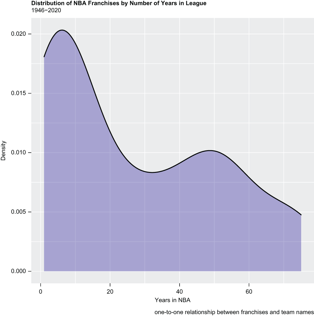
Inspect the franchise-years density plot to see the left-side concentration and longer right tail associated with the Lindy effect. section 15.0

