A risk-free return is the known return on an investment whose maturity matches the investment horizon and whose cash flows contain no intermediate coupons. Under these conditions, the asset has zero volatility. A one-month Treasury bill fits a one-month horizon; a ten-year government bond sold after one month does not, because its price may rise or fall. section 2.4
Adding a risk-free asset changes portfolio construction: combinations of it and a tangent portfolio form a capital allocation line above the efficient frontier. The investor controls risk exposure through the allocation between the two assets. section 2.4
The risk-free return enters the optimization as follows:
- Represent the risk-free asset's return as R_f and its portfolio weight as w_0. section 2.8
- Constrain total expected return with μᵀw + R_f w_0 = μ_p and total weights with 1ᵀw + w_0 = 1. section 2.8
- Eliminate w_0 to obtain excess-return terms, μ − R_f1, in the minimum-variance problem. section 2.8
- Solve the resulting equations for optimal risky-asset weights using the covariance matrix and the Lagrange multiplier. section 2.8
Blending the tangent portfolio and the risk-free asset
A portfolio with 70% in the tangent portfolio and 30% in the risk-free asset lies 70% of the way toward the tangent portfolio. A more risk-averse allocation reverses those proportions. section 2.4
Figure 2.4 Risk–reward plot with a capital allocation line
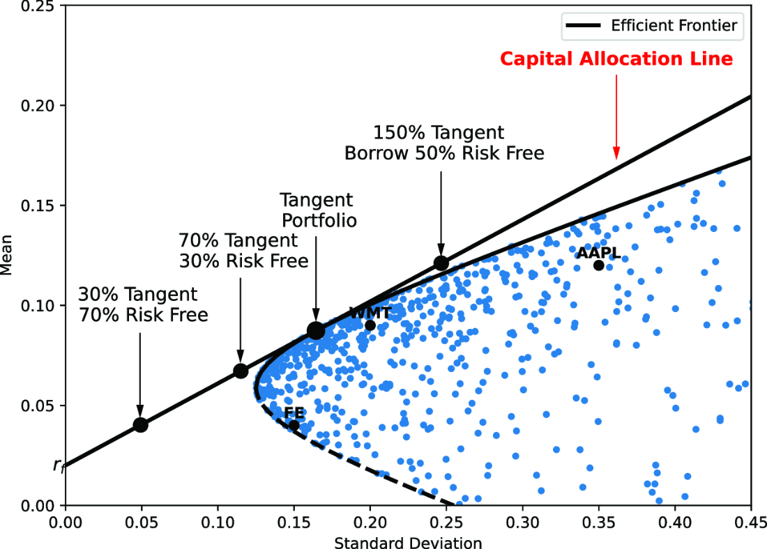
Use the risk–reward plot to see how the risk-free point connects to the tangent portfolio through the capital allocation line. section 2.4

