A sampler is the tool that walks a diffusion model from noisy latent data toward an image. It controls how noise is removed across the run; the schedule type controls how much is removed at each step. Think less magic paintbrush, more hair stylist: the tool and the size of each trim both affect the final look. section 6.0 section 6.1.2
Sampler changes are usually subtle compared with changing a checkpoint, but subtle is exactly where image polishing lives. There is no universally best choice: hold the rest of a generation fixed, try alternatives, and judge the resulting images rather than expecting a winner on paper. section 6.1.1 section 6.3
A practical sampler workflow:
- Start with an available default, then compare samplers using the same checkpoint, prompt, seed, dimensions, step count, schedule, and CFG scale. section 6.2.2
- Test DDIM, Euler, and DPM++ 2M as representative methods from different periods of diffusion sampling. section 6.1.2 section 6.2.1
- Increase sampling steps when a low-step result looks weak or samplers disagree sharply; differences can become nearly invisible at higher counts. section 6.2.2
- Treat high CFG scale and low step counts as a combination worth testing carefully, especially with higher-order samplers. section 6.2.2
- Tune schedule type late, after larger configuration decisions, for another small aesthetic adjustment. section 6.4
A controlled sand-castle test
Generate “a sand castle on the beach” with seed 1337, 512×512 output, Karras schedule, CFG 7, and 10 steps. Compare DDIM, Euler, and DPM++ 2M. Then repeat at 30 steps: the initially noticeable differences can shrink until preference is largely subjective. section 6.2.2
Under the hood, samplers are alternative approximate ways to solve the ordinary differential equation describing how latent images change as noise is reduced. That explains why several methods exist, not why you need to become an ODE enthusiast before using the dropdown. section 6.2 section 6.2.1
Figure 6.7 Exploring 10 steps with 3 different sampling methods.
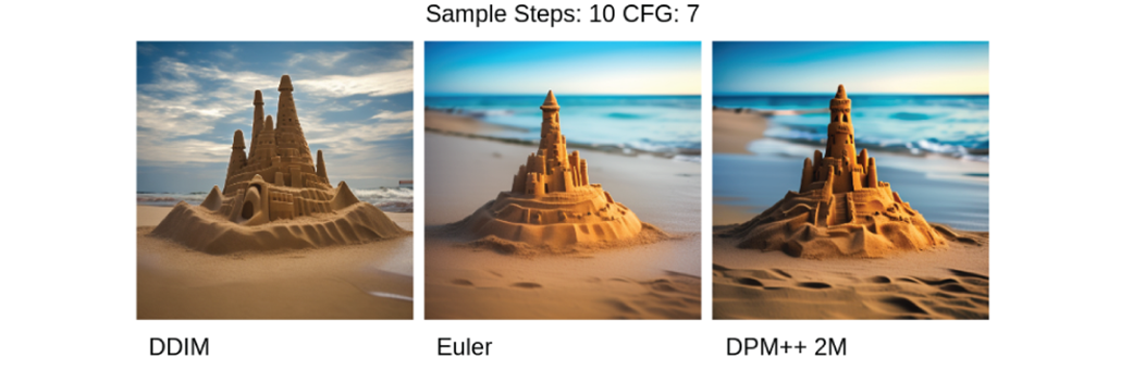
Compare the three methods at the same 10-step configuration before changing any other setting. section 6.2.2