A sampling distribution is the distribution you get by repeatedly drawing samples of the same size from a population, calculating one statistic from each sample, and examining those results. For example, one sample mean is a point estimate; many sample means reveal how that estimate tends to vary. section 5.2
Imagine 3,210 recorded tornado widths. Draw 45 widths at random, calculate their mean, and repeat that 1,000 times. A histogram of those 1,000 means is a sampling distribution of the mean. It can look bell-shaped even when the original tornado-width data are strongly right-skewed. section 4.9
Figure 4.13 Tornado width sample means plotted as a histogram
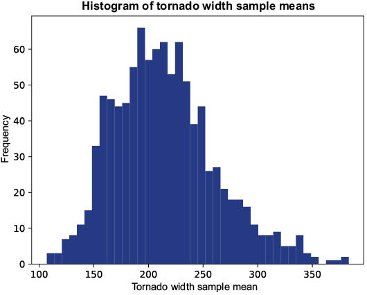
Compare the histogram of repeated sample means with the skewed population data: averaging samples produces a much more regular pattern. section 4.9
For sample means, the central limit theorem links the sampling distribution to the population: its center is the population mean, while its spread is the population standard deviation divided by the square root of sample size. That spread shrinks as samples get larger, so sample means cluster more tightly around the population mean. section 4.9 section 5.1
How sample size changes a probability
With population mean 98.2°F, population standard deviation 0.73, and samples of 31, the sampling distribution can be modeled as normal to estimate a 6.36% probability that a sample mean is below 98°F. Increasing n from 31 to 60 or 100 narrows the curve and reduces tail probability. section 5.1
Sampling distributions also apply to proportions. Repeated, broadly sampled polls can produce a distribution of sample proportions, letting you ask how likely a result such as 55% or fewer is for samples of 100 people. Biased venues can distort the result, so sampling should be as unbiased as possible. section 5.7
For proportions, a normal approximation uses the population proportion as its center and a standard error in place of a standard deviation. Rules of thumb such as n × p ≥ 5 and n × (1 − p) ≥ 5 help make that approximation reasonably accurate. In practice, population values are often unavailable, which is why sampling distributions lead into confidence intervals. section 5.7 section 5.2
