Simulation executes a model to estimate how a system’s state will change under specified inputs and conditions. A model describes relationships among inputs, internal states, and outputs; running it lets you ask what could happen rather than merely inspect what is happening. In a digital twin, observations from the physical system keep those estimates tied to current conditions. section 9.1 section 9.1.1
Choose an approach that matches how the system changes:
- For continuous changes, such as room temperature or tank level, evolve the modeled state over time while varying inputs and initial conditions. section 9.0 section 9.1.2
- For discrete events, such as jobs entering a queue or machines stopping, advance between events. SimPy schedules processes and jumps directly to the next event rather than calculating through idle periods. section 9.0 section 9.4.2
- For structural behavior, physics-based methods such as finite element analysis can support condition monitoring; reduced-basis FEA makes some industrial simulations fast enough for operational use. section 9.5.2
Build the loop in order: define the decision and desired outcome, collect and transport relevant data, build the model, run scenarios, then use the results to guide action. Sensor readings can initialize a run; comparing predicted outputs with observed outputs helps calibrate and validate the model. This matters because fixed assumptions can drift away from actual operating conditions. section 1.6 section 9.1.1 section 9.1.2
Predict when a tank will drain
Define a tank’s geometry, outlet, initial water level, and fluid behavior in OpenModelica. Run the model to plot water level over six hours, then rerun it with a sensor-measured starting level. The OpenModelica result predicts a longer drain time than an idealized Python model because its fluid model accounts for effects including viscosity and turbulence. The difference is a reminder to check what each model assumes before acting on its prediction. section 9.3.2
Figure 9.5 Output of a simulation run for the tank model, with an initial water height of 2 meters, showing the change in level over time
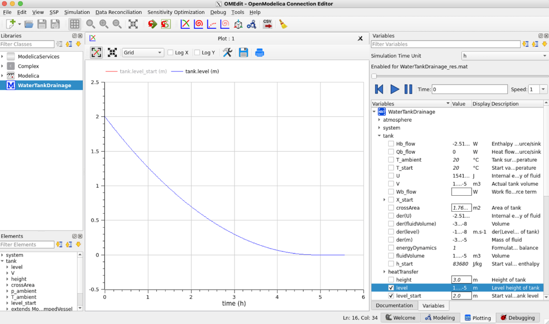
The tank-level plot makes the predicted change over time visible for a specified starting height. section 9.3.2
Test a household power limit
Model a washer, dryer, dishwasher, and electric vehicle as SimPy processes sharing a 7 kW power supply. Each appliance requests power, runs for a variable duration, and returns that capacity when finished. Simulating these events shows how a shared constraint affects when electricity-consuming chores can complete. section 9.4.2
Simulation reduces the risk of testing changes on a live system, but predictions still depend on the model and its data. At industrial scale, maintaining trustworthy results requires calibrated models, data pipelines, compute capacity, and governance as assets and operating conditions change. section 1.4.3 section 9.7.2