When a demand plan needs a fair, practical comparison point, local averaging offers a simple benchmark. A moving average predicts the next value by averaging demand from a recent fixed number of periods; averaging the last three to six periods often performs well. section 10.1.2
Use several window sizes rather than accepting an artificially weak benchmark. Compare forecasts at the same lag: a forecast made three months ahead should be compared with a moving average using demand from three months earlier. Continue tracking both over time instead of treating the comparison as a one-off test. section 10.1.2
Local averaging is especially useful when:
- A simple, free, and fair benchmark is needed for forecasting accuracy. section 10.3
- A consensus forecast needs to be tested against past sales rather than judged in isolation. section 12.2.4
- Promotion-driven demand may allow an informed forecast to outperform the benchmark because the average contains no promotion information. section 12.2.4
A practical benchmark check
Run a moving average over past sales and compare its accuracy with the consensus forecast. If the consensus forecast improves on the benchmark by less than 5%, treat that gap as a signal that the planning process may have room to improve. For a six-month horizon involving planners, sales, and management, evaluating forecast value added requires tracking multiple forecast versions for each lag. section 12.2.4
Figure 10.3 Forecast vs. benchmark; see metrics in table 10.2.
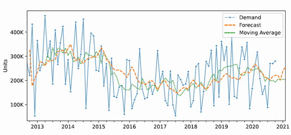
Inspect the forecast-versus-benchmark figure and its associated metrics when comparing local averaging with another forecasting approach. section 10.1.2