Suppose an algorithm works well on a small input but runs out of memory on a large one. Space complexity describes how the memory it needs grows as the input grows. It sits alongside time complexity when comparing algorithms, especially where inputs are large or memory is limited. section 1.3.1 section 1.3
Ask what the algorithm must keep while it runs: stored elements, a queue or stack, a set of visited nodes, or a table of results. Then relate that storage to input size using Big O notation. A fast operation does not necessarily mean small overall memory use. section 1.3 section 1.3.1 section 1.4.3
A few examples make the scale easier to see:
- A stack holding N elements has O(N) space complexity, even though pushing or popping its top element takes O(1) time. section 1.4.3
- Breadth-first search of a tree uses a queue that can hold an entire level: O(W) space for maximum width W. Depth-first search uses O(D) space for maximum depth D. section 1.4.4
- Breadth-first and depth-first graph traversals use a visited set to prevent cycling back through nodes. That set can grow to V vertices, giving the stated O(V) space bound. section 1.4.5
Figure 1.11 Traversal paths shown through a network with a cycle. Left: Depth-First Search (DFS) traces deep pathways until it detects dead-ends and mismatches. Right: A Breadth-First Search (BFS) expands to all neigboring or adjacent nodes. Both traversals use a visited set to track already visited nodes to avoid infinite loops.
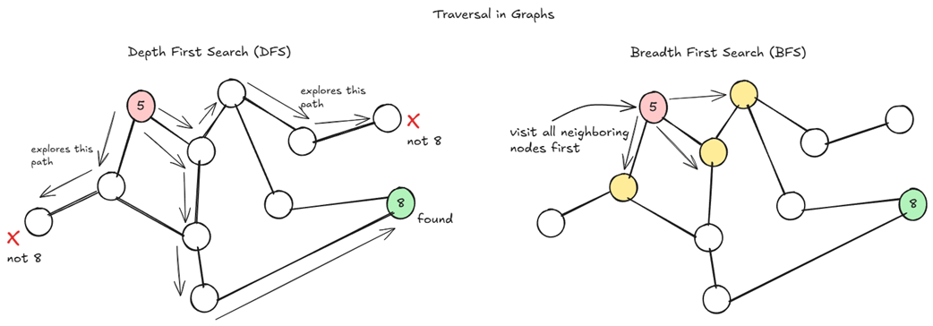
The traversal paths show why both searches must remember visited nodes when a graph contains a cycle. section 1.4.5
When a table becomes too large
A two-dimensional knapsack table has O(n×W) space complexity, where n is the number of items and W is the capacity limit. Even with few items, a very large W can make the table impractical. Because each calculation uses values from the preceding row, a one-dimensional array can reduce memory use for this formulation. section 7.3
The representation matters too. Floyd–Warshall keeps one V×V distance grid and has O(V²) space complexity; it can update that grid without retaining every earlier version. Push–Relabel has O(V²) space with static capacity and flow matrices, or O(V+E) with adjacency lists. When choosing an approach, check both its memory bound and the quantities that make that bound grow. section 9.1 section 10.4