A spatial method combines data across neighborhoods defined by a graph’s connections. Think of moving a convolutional filter across an image: each position supplies a local patch. On a graph, the comparable window is a node and its linked neighbors, not a fixed grid of pixels. This makes spatial convolution useful for learning local patterns when connections, rather than pixel positions, define what is nearby. section 3.4.1 section 3.4.2
Figure 3.12 A comparison of convolution over grid data (left; e.g., a 2D image) and over a graph (right).
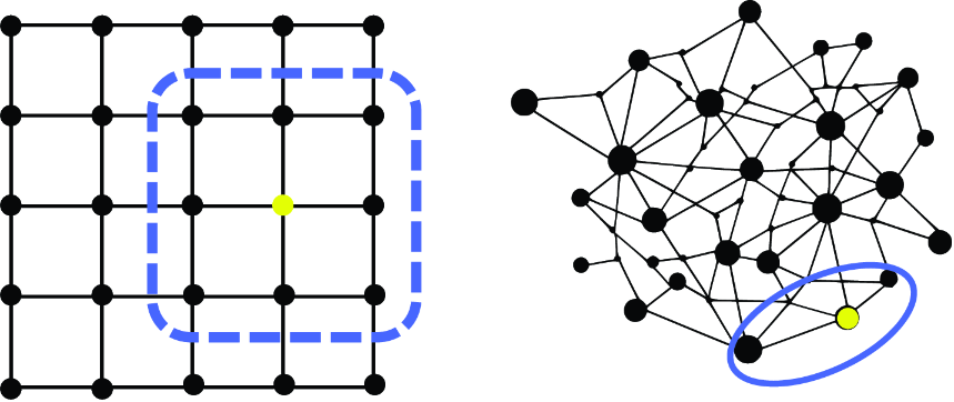
Compare the fixed image grid with the connected graph to see why a graph neighborhood replaces a fixed-size image patch. section 3.4.1
A spatial layer can be understood as a message-passing pipeline:
- Aggregate information from connected neighbors. section 3.4.2
- Transform the collected information into features, then update node or edge features. section 3.4.2
- Repeat layers to include information from more hops away; test depth because overly deep models can make node features too similar. section 3.4.2 section 3.6
Spatial and spectral methods are alternative ways to describe graph convolution, not a strict either-or choice. Spatial methods emphasize neighborhood aggregation; spectral methods filter graph signals. A spectrally derived operation can sometimes be interpreted spatially. Spatial methods are generally described as less computationally complex and less restricted, but aggregation choice and model configuration still need empirical testing. section 3.4.5 section 3.6
Product co-purchase graph
Products purchased in the same transaction form linked nodes. To predict product categories, a model can combine a product’s features with information from its connected products. Mean, max, and sum aggregation offer different ways to combine those neighborhood messages; testing them helps identify what works for the graph. section 3.6
