Sum of squares measures how far a model’s predictions are from the observed data. It squares each residual—the difference between an actual value and a predicted value—then adds the squared differences together. section 7.9
To score a regression line:
- Calculate each predicted y-value from the line. section 7.9
- Subtract each prediction from its actual y-value to get a residual. section 7.9
- Square the residuals and add them; the result is the loss. section 7.9
- Prefer a smaller sum, because it indicates that the data lies closer overall to the line. section 7.9
A sports-drink regression line
For a sports-drink dataset, a line using m = 9.74 and b = -405.26 produces a sum of squares by comparing every observed sales value with its prediction. Regression searches for coefficient values that minimize this loss, but a zero score from an overly flexible model can overfit known data and predict new data poorly. section 7.9 section 7.10
import numpy as np

x = np.array([51.5, 55.1, 63.0, 71.2, 73.0, 77.1,
    88.1, 91.2, 93.0, 101.6])

y = np.array([100.98, 137.44, 237.8, 254.96, 263.45,
    353.89, 450.32, 521.34, 503.13, 573.91])

m = 9.74  #1
b = -405.26  #1

sum_of_squares = 0  #2
for i in range(len(x)):  #2
    actual_y = y[i]
    predicted_y = m * x[i] + b
    sum_of_squares += (actual_y - predicted_y) ** 2

print(f"Sum of squares: {sum_of_squares:.2f}")  #3
Run the Python listing to calculate the sum of squared residuals for a chosen regression line. section 7.9
Figure 7.8 A 3D plot showing the sum of squares for different m and b values. We are trying to find the m and b values at the lowest point in this valley.
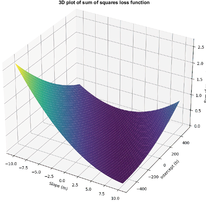
Inspect the loss surface as slope and intercept change; the lowest point represents the coefficient combination with the smallest sum of squares. section 7.9
