Transposed convolution

As explained in Inside Deep Learning: Math, Algorithms, Models

A convolution-like operation used to increase spatial resolution in a tensor, often to undo downsampling from pooling in dense prediction models.

Transposed convolution expands a tensor’s spatial dimensions after downsampling. It supports dense prediction tasks such as image segmentation, where the model must produce one prediction per pixel. Pooling reduces memory use and increases the receptive field; a later transposed convolution restores width and height. section 8.0 section 8.2

A normal convolution combines multiple input values into each output location and usually shrinks the spatial dimensions. A transposed convolution reverses this mapping: each input contributes to several output locations, and overlapping contributions are added. The interior calculation can match a regular convolution, while border handling produces expansion instead of shrinkage. section 8.2

Stride controls how far the expansion moves across the output:

• With stride 1, the filter advances one output position at a time. section 8.2
• With stride 2, the transposed convolution can double height and width, countering a factor-of-two reduction from pooling. section 8.2
• Padding, kernel size, stride, and output padding jointly determine the exact output shape. section 8.2.1

Undoing one pooling operation in PyTorch

A segmentation network can shrink features with nn.MaxPool2d(2), then restore their spatial dimensions with nn.ConvTranspose2d(2*n_filters, n_filters, (3,3), padding=1, output_padding=1, stride=2). Batch normalization, a LeakyReLU, further convolutional layers, and a final nn.Conv2d produce the mask. This arrangement produced more solid regions, somewhat better edge cases, slightly lower validation error, and faster progress in the reported experiment. section 8.2.1

U-Net uses transposed convolution in a bottleneck path: pooled, low-resolution features are expanded to the original width and height, then combined with earlier full-resolution features through skip connections. This combines broad object context with fine borders. section 8.3

Figure 8.3 Step-by-step calculation of a transposed convolution. The green region on the left shows which part of the input is being used, and the orange on the right shows which part of the output is being altered. At every step, the input is multiplied by the filter and added to the output at the given location. Because the input expands by the size of the filter, the size of the output is larger than that of the input.

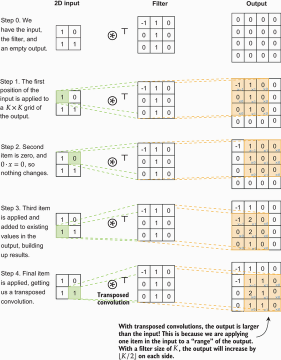
Follow the step-by-step 2×2 calculation to see each input value multiplied by the filter and added into overlapping output locations. section 8.2

Transposed convolutions can create unevenly spaced artifacts. An alternative is nn.Upsample, optional nn.ReflectionPad2d for shape correction, and a normal nn.Conv2d for channel mixing; compare both designs empirically. section 8.6

How Inside Deep Learning: Math, Algorithms, Models covers it

How deep it goes

Explains overlapping contributions, borders, stride, PyTorch parameters, architectures, and artifacts without deriving gradients.

Examples

Uses 2×2 mapping diagrams, a pooled segmentation model, U-Net blocks, autoencoder exercises, and a two-stage GAN generator.

What it assumes

Builds on normal convolution, filter stride, max pooling, feature maps, and basic PyTorch sequential networks.

What you can do after

Builds PyTorch segmentation or generator layers that restore spatial size after pooling and evaluates artifact-reduction alternatives.

How it connects

Connects convolution, max pooling, image segmentation, U-Net, skip connections, convolutional autoencoders, and generative adversarial networks.

liveBookmanning.com

Read Inside Deep Learning: Math, Algorithms, Models on liveBook Get the book at manning.com

Also explained in

• 

  liveBookmanning.com
  Learn Generative AI with PyTorchThe 2D computation performed by a transposed convolutional layer to expand an image or feature map.
• 

  liveBookmanning.com
  Build a Text-to-Image Generator (from Scratch)A transposed convolutional layer increases spatial resolution by applying a learned convolution-like operation that can expand spatial dimensions.
• 

  liveBookmanning.com
  Math and Architectures of Deep LearningA convolution-like operation often described via the transpose of the convolution matrix, used here as a motivation for understanding the matrix form of convolution.
• 

  liveBookmanning.com
  Grokking AI Algorithms, Second EditionA transposed convolution is a learnable convolutional operation that projects a lower-resolution representation into a higher-resolution output space.

Compare how 5 books explain transposed convolution →

Related concepts

• up blockused by · An up block is a U-Net component that increases spatial resolution through operations such as transposed convolution.
• upsamplingimplements · Upsampling is a process that increases the number, density, or spatial or temporal resolution of samples or values in a dataset or representation by adding, duplicating, or estimating them.
• convolution kerneluses · A convolution kernel is a small array or tensor of weights applied across local input regions to compute weighted responses and detect or transform patterns.
• convolutional layercontrasts with · A convolutional layer is a neural-network layer that applies shared learned filters to local regions of structured input to produce feature representations.
• decodeused by · Decoding is the process of transforming an encoded or internal representation into an interpretable or target-form output.

This explainer was generated by Manning's knowledge graph from the text of Inside Deep Learning: Math, Algorithms, Models. The section links point to the parts of the book it draws on.