Treatment effect heterogeneity

As explained in Causal Inference for Data Science

Treatment effect heterogeneity is variation in a treatment's causal effect across units, covariate levels, or subpopulations.

A treatment does not always work equally well for everyone. Suppose a travel agency raises a flight ticket price by $5: the same increase may reduce holiday sales less than sales outside the holiday season. When a causal effect varies across seasons, covariate levels, or subpopulations, it is a heterogeneous treatment effect. section 8.1.4

An ordinary partially linear model assumes one constant treatment effect: sales = β price + g(season) + V. To measure effects for particular values of a variable X, estimate a conditional average treatment effect (CATE), such as the average effect of price separately by season. section 8.1.4

Interactions represent heterogeneous effects

A linear model without interactions, L = a + bP + cS + U, gives every season the same price slope. Adding an interaction, L = a + bP + cS + dP × S + U, allows the slope to change with season: it is b when S = 0 and b + d when S = 1. section 8.1.4

Double machine learning can estimate heterogeneous effects after flexible predictive modeling. It removes confounder influence from both treatment and outcome, then uses the remaining residual variation to estimate causal effects for different subpopulations, such as loyal and infrequent clients. section 8.1 section 8.0

Heterogeneity also changes what can be learned from treated and untreated units. With chatbot use, the effect among treated customers may differ from the population effect; without homogeneity, ATE and ATET need not agree. section 10.4

Graph used throughout this chapter. C denotes the vector of confounders, D stands for decision, and O is the outcome.

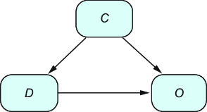
Use the causal graph to identify confounders, treatment, and outcome before estimating heterogeneous effects. section 8.1

How Causal Inference for Data Science covers it

How deep it goes

Defines CATE, derives interaction terms, and connects heterogeneity to DML and ATE-versus-ATET differences.

Examples

Uses seasonal flight pricing and chatbot adoption to contrast population, treated-group, and subgroup effects.

What it assumes

Assumes familiarity with causal effects, confounders, linear models, and average treatment effects.

What you can do after

Apply interaction models or DoubleML to estimate causal effects that vary across observed subpopulations.

How it connects

Connects conditional average treatment effects, interactions, double machine learning, confounding, potential outcomes, ATE, and ATET.

liveBookmanning.com

Read Causal Inference for Data Science on liveBook Get the book at manning.com

Related concepts

• double machine learningproduced by · Double machine learning is a causal-effect estimation method that uses machine-learning nuisance models with orthogonalized estimation to reduce bias from nuisance-function errors.
• estimatorcontrasts with · An estimator is a rule, procedure, or computational model that uses data or measurements to produce an estimate of an unknown quantity, parameter, prediction, or state.

This explainer was generated by Manning's knowledge graph from the text of Causal Inference for Data Science. The section links point to the parts of the book it draws on.