Double machine learning

As explained in Causal Inference for Data Science

Double machine learning is a causal estimation technique that combines machine-learning nuisance models with orthogonalized effect estimation to reduce bias from estimating those nuisance components.

Double machine learning (DML) estimates the causal effect of a continuous decision variable when confounders may affect both the decision and outcome through complex nonlinear relationships. It is a more flexible follow-up to a linear baseline when accuracy matters. section 8.0 section 8.1

The core idea is to use two machine-learning models: one predicts the decision from confounders, and another predicts the outcome from confounders. DML then estimates the decision’s effect using what remains after those predictions—the residual variation not explained by the confounders. section 8.1

A common version is the partially linear model (PLM). It allows nonlinear confounder relationships while keeping the decision–outcome effect linear and constant: a one-unit decision change has the same estimated effect at every decision level. section 8.1.2

A practical DML workflow is to:

• Choose confounders using causal reasoning, such as the back-door criterion, and ensure relevant confounders were measured. section 8.1 section 8.6
• Fit machine-learning nuisance models for the decision and outcome from the confounders. section 8.1.2
• Use cross-fitting, training models on one data split and estimating residuals on another, then rotate the splits. section 8.1.3
• Estimate the causal effect from the residualized decision and outcome, with uncertainty intervals where available. section 8.1 section 8.6

Ticket pricing and sales

An airline wants the effect of ticket price on sales. Seasonality influences both prices and sales, potentially nonlinearly. DML can model those seasonal patterns flexibly while estimating a linear price effect; if the price effect itself differs by season, the partially linear model is insufficient. section 8.1 section 8.1.2

Figure 8.1 Steps to run the DML algorithm. The main goal of this algorithm is to first get rid of the influence of confounder C on both the decision and outcome variables. This is done using two predictive models. What remains after their predictions, called residuals, is used to estimate the causal effect from D to O.

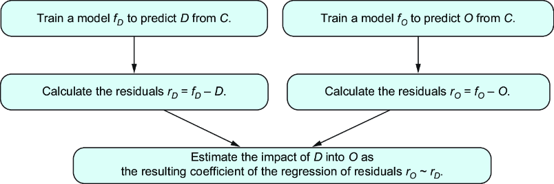
Follow the two predictive-model steps and see how their residuals become the inputs for causal-effect estimation. section 8.1

DML is not a substitute for causal design. Its reliability still depends on adjusting for the relevant measured confounders; flexible prediction alone cannot establish that requirement. section 8.6

How Causal Inference for Data Science covers it

How deep it goes

Explains residualization and partially linear assumptions, while deferring library-specific instruction to external documentation.

Examples

Uses airline ticket pricing and sales, plus 401(k) enrollment and net financial assets.

What it assumes

Assumes relevant confounders are measured or selected with tools such as the back-door criterion.

What you can do after

Apply it via DoubleMLPLR in R or Python with models predicting treatment and outcome from confounders.

How it connects

Connects confounders, the back-door criterion, linear models, cross-fitting, confidence intervals, and doubly robust estimation.

liveBookmanning.com

Read Causal Inference for Data Science on liveBook Get the book at manning.com

Related concepts

• DoubleMLimplemented by · DoubleML is an open-source software library for estimating causal effects with double machine learning and related methods in R and Python.
• Frisch–Waugh–Lovell theoremuses · The Frisch–Waugh–Lovell theorem states that the coefficient of a variable in a multiple linear regression equals the coefficient obtained by regressing residualized outcomes on residualized predictors.
• estimatoruses · An estimator is a rule, procedure, or computational model that uses data or measurements to produce an estimate of an unknown quantity, parameter, prediction, or state.
• machine learninguses · Machine learning is a field of computational methods in which systems learn patterns or relationships from data to make predictions, decisions, or other outputs.
• backdoor identificationkind of · Backdoor identification is the identification of a causal effect by adjusting for variables that block noncausal backdoor paths between an exposure and an outcome.
• orthogonalizationkind of · Orthogonalization is a causal estimation technique that reduces the influence of nuisance-model estimation errors on a target parameter estimate.

This explainer was generated by Manning's knowledge graph from the text of Causal Inference for Data Science. The section links point to the parts of the book it draws on.