A uniform distribution assigns equal likelihood to its possible outcomes. For a finite set of discrete values, each value has probability 1 divided by the number of values. A fair six-sided die therefore gives each face probability 1/6. This discrete case is distinct from a continuous uniform distribution, which is not developed here. section 3.1.3
To use a discrete uniform model:
- Specify the finite set of possible values and check that each is equally likely. Their probabilities must sum to 1. section 3.1.3
- For consecutive integers from a through b, count b − a + 1 outcomes; each has probability 1/(b − a + 1). A plot of their probabilities is flat, or rectangular. section 3.1.3
- Keep equal likelihood within one draw separate from independence between draws. A previous die roll does not change the probabilities on the next roll. section 3.3.2
Generate and check a flat-digit baseline
In Python, `np.random.randint(1, 10, size=1000)` generates 1,000 integers from 1 through 9. Group the results by value and count them to inspect the observed frequencies. Each digit has the same modeled probability, but the counts need not match: one run produced counts ranging from 101 to 130, rather than exactly 111 per digit. Treat the flat pattern as an expectation, not a guarantee for a finite sample. section 12.3.1 section 12.3.3
Figure 12.2 A uniform distribution of 1,000 records on top and a random distribution of 1,000 records on the bottom. Many numeric data sets take on one of these two probability distributions. In a Benford distribution, 1s, 2s, and 3s represent more than 60% of the occurrences, but in both these distributions, those digits represent barely 30% of the occurrences.
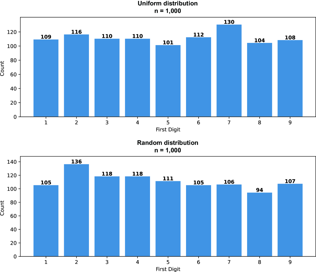
Compare the roughly flat digit counts with Benford’s leading-digit pattern, where smaller digits occur more often. The contrast helps test whether a uniform baseline is appropriate for numeric data. section 12.3.3