Unobserved confounding

As explained in Causal Inference for Data Science

An unobserved confounder is a confounding variable that influences treatment and outcome but is not measured or available in the data.

An unobserved confounder influences both treatment and outcome but is not measured or available in the data. This creates a practical causal problem: the treatment-outcome association mixes the treatment effect with the confounder’s influence. section 2.5.3

Kidney treatment decisions

Suppose doctors choose a kidney-stone treatment using stone size, but the software never stored stone size. The adjustment formula requires P(O | T, C) and P(C); without any information about C, the causal effect of T on O cannot be estimated directly. Omitting a relevant confounder can even reverse the treatment choice, as illustrated by Simpson’s paradox. section 2.5.3

Figure 2.12 Graph with an unobserved confounder (we don’t have data about this variable).

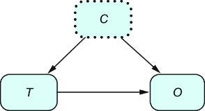
A causal graph marks the unavailable confounder with dashed lines, making the missing adjustment information explicit. section 2.5.3

Treat unobserved confounding as a limitation rather than an ordinary missing-data detail:

• State explicitly when relevant confounders may be missing, and communicate that assumption to people relying on the analysis. section 2.5.3
• Do not assume that adjusting for observed variables automatically removes bias; more complex graphs may contain relationships among observed and unobserved confounders. section 2.5.9
• Consider instrumental variables when the adjustment formula cannot be applied because confounders are unobserved, but only when the required graph structure and assumptions hold. section 9.0

Synthetic instrumental-variable check

A synthetic dataset contains an unobserved binary confounder affecting treatment and outcome. The true treatment effect is −2, while naive regression and a difference in means estimate about 1. An instrumental-variable estimate gives −1.8898, closer to the true effect under the stated assumptions. section 9.3

How Causal Inference for Data Science covers it

How deep it goes

Explains the missing adjustment probabilities and practical risk, but defers sensitivity-analysis methods to specialized treatment.

Examples

Uses kidney-stone treatment, shoe pricing, chatbot usage, and synthetic binary-confounder data to expose the problem.

What it assumes

Assumes treatment, outcome, confounder, causal graphs, and the adjustment formula, while illustrating their failure through concrete examples.

What you can do after

Diagnose causal analyses for missing confounders and consider instrumental variables when their assumptions and graph structure apply.

How it connects

Connects confounding with adjustment formula, Simpson’s paradox, causal graphs, average treatment effects, and instrumental variables.

liveBookmanning.com

Read Causal Inference for Data Science on liveBook Get the book at manning.com

Related concepts

• confounderkind of · A confounder is a variable associated with both an explanatory or treatment variable and an outcome, whose influence can distort their apparent relationship or estimated causal effect.
• treatment effectcontrasts with · A treatment effect is the difference in an outcome attributable to receiving an intervention or exposure rather than a comparison condition.
• instrumental variableaddressed by · An instrumental variable is a variable that affects a treatment or exposure while influencing an outcome only through that treatment or exposure, under causal identifying assumptions.

This explainer was generated by Manning's knowledge graph from the text of Causal Inference for Data Science. The section links point to the parts of the book it draws on.