An update rule adjusts a predicted belief about a hidden state after a new observation arrives. It answers: given what we just measured, how should we revise our estimate? In a state-space model, prediction comes first; the update then uses the observation model and Bayes’ theorem to correct that prediction. section 9.3 section 9.8
A Gaussian update follows this cycle:
- Predict the next latent-state mean from the previous state. section 9.8
- Increase the predicted state variance by the state-transition noise variance S. section 9.8
- Predict the next observation variance by adding observational noise R. section 9.8
- Compute the Kalman gain, K = next_x_var / (next_x_var + R), to balance model uncertainty against measurement noise. section 9.8 section 9.15
- Move the state mean toward the observed value by K times the residual, then reduce variance to (1 − K) times the predicted variance. section 9.8
Updating a noisy time-series estimate
For a changing CO₂ concentration, the filter first predicts the next latent concentration and then compares that prediction with the newly measured value. A larger Kalman gain pulls the estimate more strongly toward the measurement; greater measurement noise reduces that pull. In NumPy, the update is represented by: K = next_x_var / (next_x_var + R); x_mean[i] = next_x_mean + K * (y[i] - next_x_mean); x_var[i] = (1 - K) * next_x_var. section 9.3
Figure 9.4 The diagram of a filter algorithm, which alternates between the prediction step and the update step to recursively generate predictions for a time series.
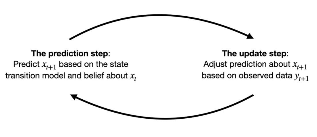
The diagram makes the update rule’s position in the recurring predict-then-correct filter cycle easy to see. section 9.3