concept algorithm in category machine learning
This is an excerpt from Manning's book Machine Learning with TensorFlow, Second Edition.
Likewise, we see that the sum of two even numbers is also an even number: 2m + 2n = 2(m + n). And lastly, we also deduce that the sum of an even with an odd is an odd number: 2m + (2n + 1) = 2(m + n) + 1. Figure 1.2 presents this logic more clearly.
The code in listing 2.9 is a simple TensorFlow program that demonstrates how to use variables. It updates a variable whenever sequential data abruptly increases in value. Think about recording measurements of a neuron’s activity over time. This piece of code can detect when the neuron’s activity suddenly spikes. Of course, the algorithm is an oversimplification for didactic purposes.
Listing 3.5 Evaluating regularization parameters
import tensorflow as tf                      #A
import numpy as np                           #A
import matplotlib.pyplot as plt              #A

learning_rate = 0.001                        #A
training_epochs = 1000                       #A
reg_lambda = 0.                              #A

x_dataset = np.linspace(-1, 1, 100)                             #B

num_coeffs = 9                                                  #B
y_dataset_params = [0.] * num_coeffs                            #B
y_dataset_params[2] = 1                                         #B
y_dataset = 0                                                   #B
for i in range(num_coeffs):                                     #B
    y_dataset += y_dataset_params[i] * np.power(x_dataset, i)   #B
y_dataset += np.random.randn(*x_dataset.shape) * 0.3            #B

(x_train, x_test, y_train, y_test) = split_dataset(x_dataset, y_dataset, 0.7)#C

X = tf.placeholder(tf.float32)        #D
Y = tf.placeholder(tf.float32)        #D

def model(X, w):                                      #E
    terms = []                                        #E
    for i in range(num_coeffs):                       #E
        term = tf.multiply(w[i], tf.pow(X, i))        #E
        terms.append(term)                            #E
    return tf.add_n(terms)                            #E

w = tf.Variable([0.] * num_coeffs, name="parameters")   #F
y_model = model(X, w)                                     #F
cost = tf.div(tf.add(tf.reduce_sum(tf.square(Y-y_model)),  #F
                     tf.multiply(reg_lambda, tf.reduce_sum(tf.square(w)))), #F
              2*x_train.size)                                              #F
train_op = tf.train.GradientDescentOptimizer(learning_rate).minimize(cost) #F

sess = tf.Session()                            #G
init = tf.global_variables_initializer()       #G
sess.run(init)                                 #G

for reg_lambda in np.linspace(0,1,100):                             #H
    for epoch in range(training_epochs):                            #H
        sess.run(train_op, feed_dict={X: x_train, Y: y_train})      #H
    final_cost = sess.run(cost, feed_dict={X: x_test, Y:y_test})    #H
    print('reg lambda', reg_lambda)                                 #H
    print('final cost', final_cost)                                 #H

sess.close()                                                    #I
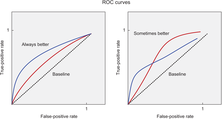
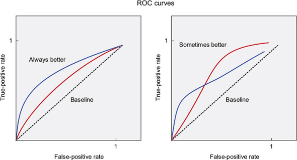
Figure 5.6 The principled way to compare algorithms is by examining their ROC curves. When the true-positive rate is greater than the false-positive rate in every situation, it’s straightforward to declare that one algorithm is dominant in terms of its performance. If the true-positive rate is less than the false-positive rate, the plot dips below the baseline shown by the dotted line.

This is an excerpt from Manning's book Grokking Machine Learning.
In most machine learning books, each algorithm is explained in a very formulaic way, normally with an error function, another formula for the derivative of the error function, and a process that will help us minimize this error function in order to get to the solution. These are the descriptions of the methods that work well in the practice, but explaining them with formulas is the equivalent of teaching someone how to drive by opening the hood and frantically pointing at different parts of the car, while reading their descriptions out of a manual. This doesn’t show what really happens, which is, the car moves forward when we press the gas pedal, and stops when we hit the breaks. In this book, we study the algorithms in a different way. We do not use error functions and derivatives. Instead, we look at what is really happening with our data, and how is it that we are modeling it.
Don’t get me wrong, I think formulas are wonderful, and when needed, we won’t shy away from them. But I don’t think they form the big picture of machine learning, and thus, we go over the algorithms in a very conceptual way that will show us what really is happening in machine learning.
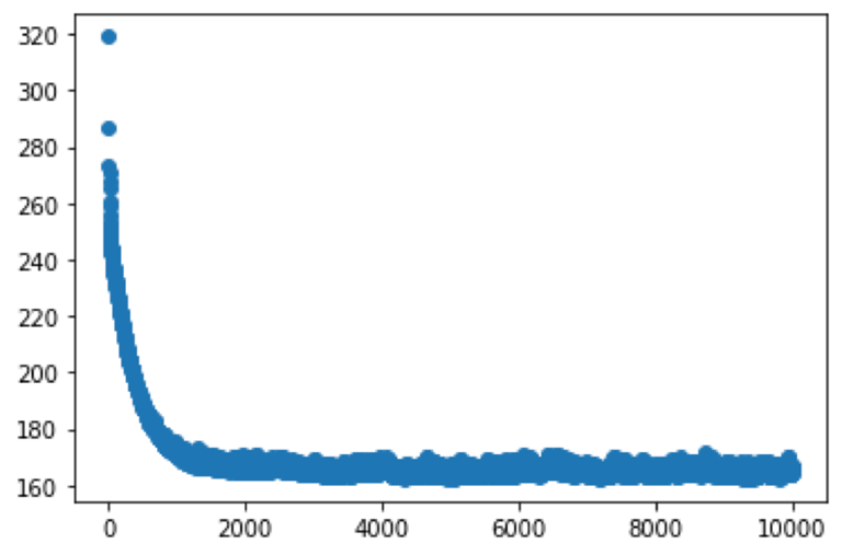
Figure 3.23. The plot of the root mean squared error for our running example. Notice how the algorithm succeeded in reducing this error after a little over 1000 iterations.
How do we code this algorithm?
Yep! By the end of this chapter we’ll code most elements of this algorithm. However, you’ll see that since the algorithm is recursive, the coding can get a bit tedious. Thus, we’ll use a very useful package called scikit learn to build decision trees with real data.

This is an excerpt from Manning's book Human-in-the-Loop Machine Learning.
This text book will help you optimize your Machine Learning algorithm strategy and your data strategy at the same time. The two are closely intertwined, and you will often get better accuracy from your models faster if you have a combined approach: algorithms and annotation are equally important and intertwined components of good Machine Learning.
For Uncertainty Sampling, you only wanted to see what was near your current decision boundary: a relatively small and well-defined feature space, like in Figure 4.1. For Diversity Sampling, we want to explore the much larger problem of every corner of our feature space, and expand the decision boundary into new parts of that space. Needless to say, the set of algorithms that you can use are more diverse and sometimes more complicated than for Uncertainty Sampling.
def get_cluster_samples(self, data, num_clusters=5, max_epochs=5, limit=5000):
    """Create clusters using cosine similarity

    Keyword arguments:
        data -- data to be clustered
        num_clusters -- the number of clusters to create
        max_epochs -- maximum number of epochs to create clusters
        limit -- sample only this many items for faster clustering (-1 = no limit)

    Creates clusters by the K-Means clustering algorithm,
    using cosine similarity instead of more common euclidean distance

    Creates clusters until converged or max_epochs passes over the data

    """

    if limit > 0:
        shuffle(data)
        data = data[:limit]

    cosine_clusters = CosineClusters(num_clusters)

    cosine_clusters.add_random_training_items(data)    #A

    for i in range(0, max_epochs):
        print("Epoch "+str(i))
        added = cosine_clusters.add_items_to_best_cluster(data)    #B
        if added == 0:
            break

    centroids = cosine_clusters.get_centroids()    #C
    outliers = cosine_clusters.get_outliers()    #D
    randoms = cosine_clusters.get_randoms(3, verbose)    #E

    return centroids + outliers + randoms

A: Initialize clusters with random assignments
B: Move each item to the cluster that it is the best fit for, and repeat
C: Sample the best-fit (centroid) from each cluster
D: Sample the biggest outlier in each cluster
E: Sample three random items from each cluster, and pass the “verbose” parameter to get an intuition for what is in each cluster.

This is an excerpt from Manning's book Machine Learning Bookcamp.
With machine learning, the problem of maintaining a hand-crafted set of rules goes away. When a new pattern emerges — for example, there's a new type of spam — we, instead of manually adjusting the existing set of rules, simply provide a machine learning algorithm with the new data. As a result, the algorithm picks up the new important patterns from the new data without damaging the old existing patterns — provided that these old patterns are still important and present in the new data.
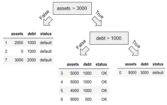
Figure 6.18 By repeating the algorithm recursively to the group on the right, we get a tree with two levels.

This is an excerpt from Manning's book Ensemble Methods for Machine Learning.
As the competition progressed and the 10% mark remained elusive, a curious phenomenon emerged among the competitors. Teams began to collaborate and share knowledge about effective feature engineering, algorithms and techniques. Inevitably, they began combining their models, blending individual approaches into powerful and sophisticated ensembles of many models. These ensembles combined the best of various diverse models and features and proved to be far more effective than any individual model.
In the previous chapter, we introduced two parallel ensemble methods: bagging and random forest. These methods (and their variants) train homogeneous ensembles, where every base estimator is trained using the same base learning algorithm. For example, in bagging classification, all the base estimators are decision tree classifiers. In this chapter, we continue exploring parallel ensemble methods, this time focusing on heterogeneous ensembles.
Heterogeneous ensemble methods use different base learning algorithms to directly ensure ensemble diversity. For example, a heterogeneous ensemble can consist of three base estimators: a decision tree, a support vector machine (SVM) and an artificial neural network. These base estimators are still trained independently of each other.
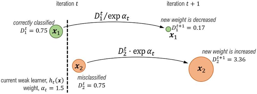
Figure 4.8. In iteration t, two training examples x1 and x2 have the same weights. x1 is correctly classified, while x2 is misclassified by the current base estimator ht(x). As the goal in the next iteration is to learn a classifier ht−1(x) that fixes the mistakes of ht(x), AdaBoost increases the weight of the misclassified example x2, while decreasing the weight of the correctly classified example x1. This allows the base learning algorithm to prioritize x2 during training in iteration t+1.

This is an excerpt from Manning's book Machine Learning with R, the tidyverse, and mlr.
Summary of the algorithms we cover in the book, whether they are supervised or unsupervised learners, and whether they can be used for classification, regression, dimension reduction, or clustering
Figure 1.6. Classification, regression, dimension reduction, and clustering. Classification and regression algorithms build models that predict categorical and continuous variables of unlabeled, new data, respectively. Dimension-reduction algorithms create a new representation of the original data in fewer dimensions and map new data onto this representation. Clustering algorithms identify clusters within the data and map new data onto these clusters.

In this section, I’ll explain the principle of the bootstrap aggregating ensemble technique, and how this is used in an algorithm called random forest. Machine learning algorithms can be sensitive to noise resulting from outliers and measurement error. If noisy data exists in our training set, then our models are more likely to have high variance when making predictions on future data. How can we train a learner that makes use of all the data available to us, but can look past this noisy data and reduce prediction variance? The answer is to use bootstrap aggregating (or bagging for short).
In this section, I’ll teach you what benchmarking is, and we’ll use it to compare the performance of several algorithms on a particular task. The classification drawer of your toolbox has lots of algorithms in it now! Experience is a great way to choose an algorithm for a particular task. But remember, we are always subject to the “no free lunch” theorem. You may find yourself surprised sometimes that a simpler algorithm outperforms a more complex one for a particular task. A good way of deciding which algorithm will perform best on a particular task is to perform a benchmarking experiment.
Cross-validate the model-building process for the algorithm that won the benchmark, performing 2,000 iterations of the random search and using holdout as the inner cross-validation strategy (inside the tuning wrapper): holdout <- makeResampleDesc("Holdout") randSearch2000 <- makeTuneControlRandom(maxit = 2000) forestWrapper2000 <- makeTuneWrapper(forest, resampling = holdout, par.set = forestParamSpace, control = randSearch2000) parallelStartSocket(cpus = detectCores()) cvWithTuning <- resample(forestWrapper2000, fuelTask, resampling = kFold) parallelStop()

This is an excerpt from Manning's book Machine Learning for Business: Using Amazon SageMaker and Jupyter.
When you implement machine learning to support Karen’s decisions, there’s little change in the management process involved for your internal customers. They continue to place orders in the same ways they always have. The machine learning algorithms simply make some of the decisions automatically, and the orders get sent to approvers and suppliers appropriately and automatically. In our view, unless the process can be cleanly separated from the other processes in your company, the optimal approach is to first implement a machine learning automation solution and then, over time, migrate these processes to your ERP systems.
In an academic paper, you want to clearly identify this threshold. In the business world, you need to weigh the benefits of accuracy against the cost of not being able to work on another project because you are spending time identifying a threshold. In Brett’s case, it is probably sufficient to compare the results of the algorithm against how well a member of Brett’s team can perform the task. If it comes out about the same, then you’ve hit the threshold.
Identify what your algorithm is trying to achieve. In Brett’s case in this chapter, the algorithm does not need to identify every erroneous line, it only needs to identify enough lines to drive the right behavior from the law firms.
This is an excerpt from Manning's book Machine Learning Systems: Designs that scale.
This brief introduction is only focused on ensuring that you’re sufficiently oriented in terms of the functionality of a machine learning system. This book is focused on the implementation of machine learning systems, not on the fundamentals of machine learning itself. Should you find yourself needing a better introduction to the techniques and algorithms used in machine learning, I recommend reading Real-World Machine Learning by Henrik Brink, Joseph W. Richards, and Mark Fetherolf (Manning, 2016).
Listing 2.15. Training a model
val numIterations = 100 #1 val model = LinearRegressionWithSGD.train(trainingParsed.rdd, numIterations) #2 #1 Max number of iterations the algorithm should run for #2 The model learned on the training set !@%STYLE%@! {"css":"{\"css\": \"font-weight: bold;\"}","target":"[[{\"line\":0,\"ch\":71},{\"line\":0,\"ch\":73}],[{\"line\":4,\"ch\":0},{\"line\":4,\"ch\":2}],[{\"line\":2,\"ch\":69},{\"line\":2,\"ch\":71}],[{\"line\":5,\"ch\":0},{\"line\":5,\"ch\":2}]]"} !@%STYLE%@!
Engineers are often excited to port legacy model-learning implementations over to Spark implementations. The code becomes simpler, the job can become much more scalable, and taking advantage of other big data tools becomes easier. Data scientists also stand to gain from this transition. When production machine learning systems use MLlib functionality, data scientists can experiment with MLlib’s wide range of algorithms. When a modeling approach works well, incorporating it into the production-data pipelines is easy.

This is an excerpt from Manning's book Machine Learning with TensorFlow.
For example, when training a model to detect cars in an image, you’ll gain an enormous performance and speed improvement if you first convert the image to grayscale. By providing some of your own bias when preprocessing the data, you end up helping the algorithm, because it won’t need to learn that colors don’t matter when detecting cars. The algorithm can instead focus on identifying shapes and textures, which will lead to much faster learning than trying to process colors as well.
Figure 4.6. The principled way to compare algorithms is by examining their ROC curves. When the true-positive rate is greater than the false-positive rate in every situation, it’s straightforward to declare that one algorithm is dominant in terms of its performance. If the true-positive rate is less than the false-positive rate, the plot dips below the baseline shown by the dotted line.
An HMM lets you understand a sequence of observations. In this weather-modeling scenario, one question you may ask is, what’s the probability of observing a certain sequence of temperature readings? We’ll answer this question by using the forward algorithm.
When you run listing 6.6, the algorithm outputs the following:

This is an excerpt from Manning's book Real-World Machine Learning.
These strategies are embodied in collections of algorithms developed over the course of recent decades by academics and practitioners in disciplines ranging from statistics, computer science, robotics, and applied mathematics, to online search, entertainment, digital advertising, and language translation. They are diverse and have various strengths and weaknesses. Some of them are classifiers. Others predict a numeric measurement. Some measure the similarity or difference of comparable entities (for example, people, machines, processes, cats, dogs). What the algorithms have in common is learning from examples (experience) and the capacity to apply what they’ve learned to new, unseen cases—the ability to generalize.
Listing 3.1. Building a logistic regression classifier with scikit-learn
from sklearn.linear_model import LogisticRegression as Model #1 def train(features, target): model = Model() model.fit(features, target) #2 return model def predict(model, new_features): preds = model.predict(new_features) #3 return preds # Assume Titanic data is loaded into titanic_feats, # titanic_target and titanic_test model = train(titanic_feats, titanic_target) #4 predictions = predict(model, titanic_test) #5 #1 - Imports the logistic regression algorithm #2 - Fits the logistic regression algorithm using features and target data #3 - Makes predictions on a new set of features using the model #4 - Returns the model built by the algorithm #5 - Returns predictions (0 or 1)
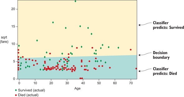
Figure 3.7. The decision boundary for the Age and sqrt(Fare) features. The diamonds show passengers who survived, whereas circles denote passengers who died. The light background denotes the combinations of Age and Fare that are predicted to yield survival. Notice that a few instances overlap the boundary. The classifier isn’t perfect, but you’re looking in only two dimensions. The algorithm on the full dataset finds this decision boundary in 10 dimensions, but that becomes harder to visualize.
For massive training sets, our recommended method of feature selection is Lasso. Lasso is an efficient linear learning algorithm that automatically searches for the most predictive subset of features. Computing the entire trace of the algorithm is efficient, allowing the user insight into the entire ordering of all the features in terms of their predictive power in the linear model. Moreover, the best subset of features, in terms of the linear model predictions, is provided.
If you’re (un)lucky enough to have such a large dataset that you can’t even fit a Lasso model, you may consider fitting the Lasso to subsets of the instances in your training set (and potentially averaging across runs of the algorithm). This can give you a good sense of which features can be removed from the model without degrading the statistical performance of your ML algorithm.
In many cases, it’s more feasible to upgrade your hardware or find more-efficient algorithms or more-efficient implementations of the algorithms you’ve chosen. But in other situations, scaling a nonlinear model is needed, and in this section we discuss a few ways to approach this.

This is an excerpt from Manning's book Algorithms of the Intelligent Web, Second Edition.
Nor is this a detailed book about algorithm design. We’ll often skim over details as to the design of algorithms and provide more intuition than a deep dive into specifics. This will allow us to cover much more ground, perhaps at the cost of some rigor. Think of each chapter as a trail of breadcrumbs leading you through the important aspects of that approach and nudging you toward resources where you can learn more.
Although many of the examples within the pages of this book are written using scikit-learn (http://scikit-learn.org), this isn’t a book about scikit-learn! That is merely the tool by which we can demonstrate the approaches presented in this book. We’ll never provide an example without at least an intuitive introduction as to why the algorithm works. In some cases we’ll go deeper, but in many cases you should continue your research outside this book.
In the previous chapter, you got your feet wet with the concept of intelligent algorithms. From this chapter onward, we’re going to concentrate on the specifics of machine-learning and predictive-analytics algorithms. If you’ve ever wondered what types of algorithms are out there and how they work, then these chapters are for you!
Note that this final assignment is exactly the means we would have chosen if we had manually performed clustering (that is, we visually determined the clusters and calculated their means); thus the algorithm has automatically determined an intelligent clustering of the data with minimal intervention from the developer!
Be aware that although the algorithm provably converges if you use the Euclidean distance function,[3] there’s no guarantee that convergence reaches a global minimum; that is, the final clustering reached may not be the best. The algorithm can be sensitive to initial starting conditions and identify different (local minima) cluster means. Consequently, in application you might consider multiple starting points, rerunning the training several times. One approach then to getting closer to the global minima is to use the average of each resultant centroid group as the starting centroids for a final run. This may put you in a better starting position to reach the best clustering. No such guarantees are given, though.
Listing 6.2. The perceptron learning algorithm (2)
Initialize w to contain random small numbers For each example j: yj(t) = Skwk(t) · xj,k #1 For each feature weight k: #2 wk(t + 1) = wk(t) + h(dj - yj(t)) · xj,k #3 #1 - Calculates the output of the perceptron given the current weights (time t) #2 - Updates the features. Note this is often done as a vector operation rather than a for loop. #3 - Features are updated only if the expected output dj and the actual output differ. If they do, we move the weight in the sign of the correct answer but a magnitude given by the corresponding input and scaled by h. h represents the speed at which the weights are updated in the algorithm. !@%STYLE%@! {"css":"{\"css\": \"font-weight: bold;\"}","target":"[[{\"line\":0,\"ch\":11},{\"line\":0,\"ch\":12}],[{\"line\":2,\"ch\":19},{\"line\":2,\"ch\":20}],[{\"line\":3,\"ch\":21},{\"line\":3,\"ch\":22}],[{\"line\":4,\"ch\":4},{\"line\":4,\"ch\":5}],[{\"line\":5,\"ch\":63},{\"line\":5,\"ch\":64}],[{\"line\":7,\"ch\":99},{\"line\":7,\"ch\":100}]]"} !@%STYLE%@!
This is an excerpt from Manning's book Introducing Data Science: Big data, machine learning, and more, using Python tools.
When you have the data in place, it’s time to extract the coveted insights. This is where you rely on the fields of machine learning, statistics, and applied mathematics. Before World War II everything needed to be calculated by hand, which severely limited the possibilities of data analysis. After World War II computers and scientific computing were developed. A single computer could do all the counting and calculations and a world of opportunities opened. Ever since this breakthrough, people only need to derive the mathematical formulas, write them in an algorithm, and load their data. With the enormous amount of data available nowadays, one computer can no longer handle the workload by itself. In fact, several algorithms developed in the previous millennium would never terminate before the end of the universe, even if you could use every computer available on Earth. This has to do with time complexity (https://en.wikipedia.org/wiki/Time_complexity). An example is trying to break a password by testing every possible combination. An example can be found at http://stackoverflow.com/questions/7055652/real-world-example-of-exponential-time-complexity. One of the biggest issues with the old algorithms is that they don’t scale well. With the amount of data we need to analyze today, this becomes problematic, and specialized frameworks and libraries are required to deal with this amount of data. The most popular machine-learning library for Python is Scikit-learn. It’s a great machine-learning toolbox, and we’ll use it later in the book. There are, of course, other Python libraries:
PyBrain for neural networks —Neural networks are learning algorithms that mimic the human brain in learning mechanics and complexity. Neural networks are often regarded as advanced and black box.
A large volume of data poses new challenges, such as overloaded memory and algorithms that never stop running. It forces you to adapt and expand your repertoire of techniques. But even when you can perform your analysis, you should take care of issues such as I/O (input/output) and CPU starvation, because these can cause speed issues. Figure 4.1 shows a mind map that will gradually unfold as we go through the steps: problems, solutions, and tips.


This is an excerpt from Manning's book Mahout in Action.
First, Mahout is an open source machine learning library from Apache. The algorithms it implements fall under the broad umbrella of machine learning or collective intelligence. This can mean many things, but at the moment for Mahout it means primarily recommender engines (collaborative filtering), clustering, and classification.
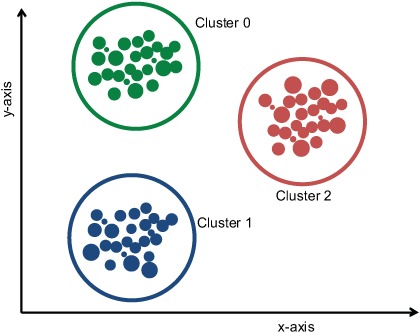
Now that you know how input data is represented as Vectors and how SequenceFiles are created as input for the clustering algorithms, you’re ready to explore the various clustering algorithms that Mahout provides. There are many clustering algorithms in Mahout, and some work well for a given data set whereas others don’t. K-means is a generic clustering algorithm that can be molded easily to fit almost all situations. It’s also simple to understand and can easily be executed on parallel computers.
Dirichlet clustering is a powerful way of getting quality clusters using known data distribution models. In Mahout, the algorithm is a pluggable framework, so different models can be created and tested. As the models become more complex there’s a chance of things slowing down on huge data sets, and at this point you’ll have to fall back on other clustering algorithms. But after seeing the output of Dirichlet clustering, you can clearly decide whether the algorithm we choose should be fuzzy or rigid, overlapping or hierarchical, whether the distance measure should be Manhattan or cosine, and what the threshold for convergence should be. Dirichlet clustering is both a data-understanding tool and a great data clustering tool.

This is an excerpt from Manning's book Collective Intelligence in Action.
Next, they allowed their users to generate content. Users could now blog about their experiences, or ask and respond to questions on message boards, or participate in building the application itself by contributing to wikis. John and Jane quickly built an algorithm that could extract tags from the unstructured content. They then matched the interests of users—gained from analyzing their interaction in the applications—with those of other users to find relevant items. They were soon able to learn enough about their users to personalize the site for each user, and to provide relevant content—targeting niche items to niche users. They could also target relevant advertisements based on the user profile and context of interaction.
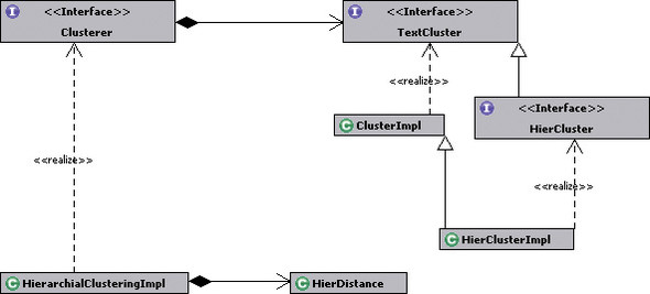
Hierarchical Agglomerative Clustering (HAC) algorithms begin by assigning a cluster to each item being clustered. Then they compute the similarity between the various clusters and create a new cluster by merging the two clusters that were most similar. This process of merging clusters continues until you’re left with only one cluster. This clustering algorithm is called agglomerative, since it continuously merges the clusters.
public void classify(Algorithm algorithm) throws Exception