An approximate distribution is a tractable probability distribution, written as q(θ), that represents an unknown target posterior p(θ | D). Variational inference chooses a family such as the Normal distribution, then adjusts its parameters to resemble the posterior. section 6.3
For a Normal approximation, the mean μ describes the center and the standard deviation σ describes uncertainty. Each pair of values creates a different q, so inference searches for the μ and σ that fit the posterior most closely. section 6.3
Shaping a balloon around jelly
Imagine the posterior as a complex blob of jelly and q as a balloon with limited shapes. Variational inference reshapes the balloon to cover the jelly efficiently. A symmetric Normal can capture the center and spread of an asymmetric Beta posterior, but cannot reproduce every feature. section 6.3
The fit is guided by the Kullback–Leibler divergence, which measures disagreement between q and the target posterior. It is zero when the distributions match and grows when q assigns substantial density where the posterior assigns little. section 6.4
During optimization:
- Gradient descent updates μ and σ to increase the evidence lower bound and reduce KL divergence. section 6.6
- A differentiable squashing function can force Normal samples into the target range, such as 0 to 1 for a Beta posterior. section 6.6
- After fitting, samples drawn from q provide approximate posterior samples. section 6.9
Figure 6.1 Unlike MCMC, which generates samples to approximate an unknown posterior, variational inference (VI) fits a simple distribution like a normal distribution to the posterior and uses the fitted distribution as the approximation.
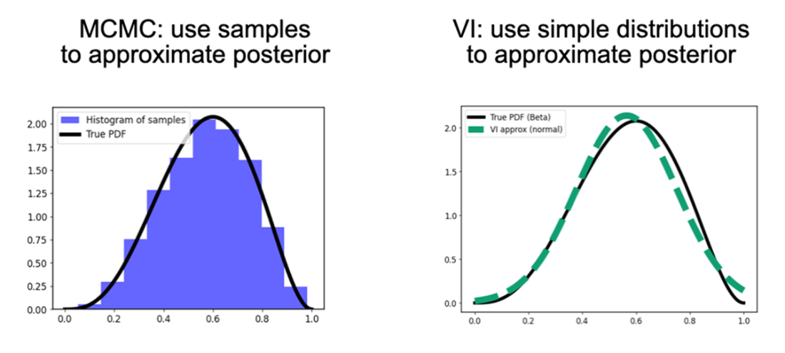
Compare sampling from a posterior with fitting a simple distribution to it. section 6.3
Figure 6.3 The evolution of the approximating distribution 𝑞 and how it’s adjusted by gradient descent throughout optimization.
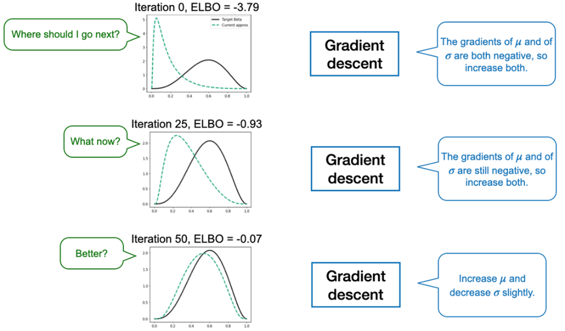
Follow how gradient descent shifts and concentrates q across optimization steps. section 6.6



