Suppose a friend tests positive for a rare illness. How likely are they to be sick? The result matters, but so does the chance of illness before the test. Bayesian statistics combines that starting probability, called the prior, with new evidence to calculate an updated probability, called the posterior. section 8.1
Bayes’ theorem answers a conditional-probability question: what is the probability of a hypothesis H given evidence E? In notation, P(H|E) = P(E|H) × P(H) / P(E). It uses the prior P(H) and the reversed conditional probability P(E|H) to find the posterior P(H|E). The denominator accounts for all ways the evidence could occur. section 8.0 section 8.2
Why a positive test may not mean illness
Among one million patients, 100 are sick. Of those, 99 test positive; another 9,999 healthy patients also test positive. So a person with a positive result has a 99 / (99 + 9,999), or about 0.98%, chance of being sick. The illness is rare enough that false positives greatly outnumber true positives. section 8.1
Figure 8.2 The tree of possibilities. Each patient can be sick or healthy. For each of the possibilities, the patient can be diagnosed as sick or healthy, which gives us four possibilities. We start with one million patients: 100 of them are sick, and the remaining 999,900 are healthy. Out of the 100 sick, one gets misdiagnosed as healthy, and the remaining 99 get correctly diagnosed as sick. Out of the 999,900 healthy patients, 9,999 get misdiagnosed as sick, and the remaining 989,901 are correctly diagnosed as healthy.
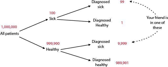
Follow the sick and healthy branches to see why a positive result includes both true positives and false positives. section 8.1
To apply the same reasoning to spam detection:
- Count spam and non-spam emails to estimate the prior probability of spam. section 8.2 section 8.3
- Use a word as evidence. In a 100-email example, 20 emails are spam; among the 20 containing “lottery,” 15 are spam. The probability of spam rises from 0.2 to 0.75 when that word is known. section 8.2
- For several words, naive Bayes multiplies word probabilities under an independence assumption, then uses Bayes’ theorem. That assumption makes the calculation manageable; it is why the model is called naive. section 8.2 section 8.4
With a real email dataset, the procedure becomes a small Python model: turn each email into a set of words, count word appearances by class, initialize counts at one to avoid zeros, and return a spam probability. Try messages with ordinary wording, promotional wording, and an unseen word; an unseen word leaves the prediction at the prior. For a rare outcome such as illness, do not rely on accuracy alone to judge a model. section 8.3 section 8.1







